Dealing with Spin in PyProcar bandsplot
This tutorial provides a comprehensive guide to handling different spin configurations when plotting band structures using PyProcar’s bandsplot function. Understanding how PyProcar handles spin is crucial for correctly interpreting and visualizing electronic band structures in magnetic materials.
Understanding Spin in PyProcar
PyProcar handles spin differently depending on the type of magnetic calculation:
Spin-Polarized Case
In spin-polarized calculations (collinear magnetism), the spin-up and spin-down channels are separate entities. This means:
There are two distinct spin channels (spin-up and spin-down)
Each spin channel has its own set of bands and eigenvalues
Each spin channel has its own corresponding orbital projections
The bands for different spins are typically plotted with different colors or styles
You can analyze spin-up and spin-down contributions independently
Non-Collinear Case
In non-collinear magnetic calculations, the situation is more complex:
Spin-up and spin-down can no longer be treated in isolation
There is only 1 spin channel (the total system)
However, there are 4 spin projections corresponding to:
Total magnetization (scalar)
sx (x-component of spin)
sy (y-component of spin)
sz (z-component of spin)
These projections provide information about the local magnetic moments and their orientations
This tutorial will demonstrate how to plot and analyze band structures for both cases.
1. Setup and Data Loading
[1]:
# Import required libraries
from pathlib import Path
import pyprocar

CURRENT_DIR = Path(".").resolve()
SPIN_POL_PATH = "data/examples/bands/spin-polarized"
NON_COLLINEAR_PATH = "data/examples/bands/non-colinear"
pyprocar.download_from_hf(relpath=SPIN_POL_PATH, output_path=CURRENT_DIR)
pyprocar.download_from_hf(relpath=NON_COLLINEAR_PATH, output_path=CURRENT_DIR)
SPIN_POL_DATA_DIR = CURRENT_DIR / SPIN_POL_PATH
NON_COLLINEAR_DATA_DIR = CURRENT_DIR / NON_COLLINEAR_PATH
print(f"Data downloaded to: {SPIN_POL_DATA_DIR}")
print(f"Data downloaded to: {NON_COLLINEAR_DATA_DIR}")
---------------------------------------------------------------------------
FileNotFoundError                         Traceback (most recent call last)
Cell In[1], line 8
      6 SPIN_POL_PATH = "data/examples/00-band_structure/spin-polarized"
      7 NON_COLLINEAR_PATH = "data/examples/00-band_structure/non-colinear"
----> 8 pyprocar.download_from_hf(relpath=SPIN_POL_PATH, output_path=CURRENT_DIR)
      9 pyprocar.download_from_hf(relpath=NON_COLLINEAR_PATH, output_path=CURRENT_DIR)
     10 SPIN_POL_DATA_DIR = CURRENT_DIR / SPIN_POL_PATH

File ~\Desktop\notebooks\Notebook\01 - Projects\Pyprocar\pyprocar\pyprocar\utils\download_examples.py:178, in download_from_hf(relpath, output_path, force)
    176 with ThreadPoolExecutor(1) as executor:
    177     future = executor.submit(download_test_data, relpath, output_path, force)
--> 178     return future.result()

File c:\Users\lllang\miniconda3\envs\pyprocar\lib\concurrent\futures\_base.py:458, in Future.result(self, timeout)
    456     raise CancelledError()
    457 elif self._state == FINISHED:
--> 458     return self.__get_result()
    459 else:
    460     raise TimeoutError()

File c:\Users\lllang\miniconda3\envs\pyprocar\lib\concurrent\futures\_base.py:403, in Future.__get_result(self)
    401 if self._exception:
    402     try:
--> 403         raise self._exception
    404     finally:
    405         # Break a reference cycle with the exception in self._exception
    406         self = None

File c:\Users\lllang\miniconda3\envs\pyprocar\lib\concurrent\futures\thread.py:58, in _WorkItem.run(self)
     55     return
     57 try:
---> 58     result = self.fn(*self.args, **self.kwargs)
     59 except BaseException as exc:
     60     self.future.set_exception(exc)

File ~\Desktop\notebooks\Notebook\01 - Projects\Pyprocar\pyprocar\pyprocar\utils\download_examples.py:155, in download_test_data(relpath, output_path, force)
    151 output_path.mkdir(parents=True, exist_ok=True)
    153 pattern = relpath + "*"
--> 155 download_dirpath = snapshot_download(
    156     repo_id=REPO_ID,
    157     repo_type=REPO_TYPE,
    158     allow_patterns=[pattern],
    159     local_dir=output_path,
    160 )
    161 download_dirpath = Path(download_dirpath)
    163 uncompress_test_data(download_dirpath / "data")

File c:\Users\lllang\miniconda3\envs\pyprocar\lib\site-packages\huggingface_hub\utils\_validators.py:114, in validate_hf_hub_args.<locals>._inner_fn(*args, **kwargs)
    111 if check_use_auth_token:
    112     kwargs = smoothly_deprecate_use_auth_token(fn_name=fn.__name__, has_token=has_token, kwargs=kwargs)
--> 114 return fn(*args, **kwargs)

File c:\Users\lllang\miniconda3\envs\pyprocar\lib\site-packages\huggingface_hub\_snapshot_download.py:324, in snapshot_download(repo_id, repo_type, revision, cache_dir, local_dir, library_name, library_version, user_agent, proxies, etag_timeout, force_download, token, local_files_only, allow_patterns, ignore_patterns, max_workers, tqdm_class, headers, endpoint, local_dir_use_symlinks, resume_download)
    320 if constants.HF_HUB_ENABLE_HF_TRANSFER:
    321     # when using hf_transfer we don't want extra parallelism
    322     # from the one hf_transfer provides
    323     for file in filtered_repo_files:
--> 324         _inner_hf_hub_download(file)
    325 else:
    326     thread_map(
    327         _inner_hf_hub_download,
    328         filtered_repo_files,
   (...)
    332         tqdm_class=tqdm_class or hf_tqdm,
    333     )

File c:\Users\lllang\miniconda3\envs\pyprocar\lib\site-packages\huggingface_hub\_snapshot_download.py:300, in snapshot_download.<locals>._inner_hf_hub_download(repo_file)
    299 def _inner_hf_hub_download(repo_file: str):
--> 300     return hf_hub_download(
    301         repo_id,
    302         filename=repo_file,
    303         repo_type=repo_type,
    304         revision=commit_hash,
    305         endpoint=endpoint,
    306         cache_dir=cache_dir,
    307         local_dir=local_dir,
    308         local_dir_use_symlinks=local_dir_use_symlinks,
    309         library_name=library_name,
    310         library_version=library_version,
    311         user_agent=user_agent,
    312         proxies=proxies,
    313         etag_timeout=etag_timeout,
    314         resume_download=resume_download,
    315         force_download=force_download,
    316         token=token,
    317         headers=headers,
    318     )

File c:\Users\lllang\miniconda3\envs\pyprocar\lib\site-packages\huggingface_hub\utils\_validators.py:114, in validate_hf_hub_args.<locals>._inner_fn(*args, **kwargs)
    111 if check_use_auth_token:
    112     kwargs = smoothly_deprecate_use_auth_token(fn_name=fn.__name__, has_token=has_token, kwargs=kwargs)
--> 114 return fn(*args, **kwargs)

File c:\Users\lllang\miniconda3\envs\pyprocar\lib\site-packages\huggingface_hub\file_download.py:988, in hf_hub_download(repo_id, filename, subfolder, repo_type, revision, library_name, library_version, cache_dir, local_dir, user_agent, force_download, proxies, etag_timeout, token, local_files_only, headers, endpoint, resume_download, force_filename, local_dir_use_symlinks)
    979     if local_dir_use_symlinks != "auto":
    980         warnings.warn(
    981             "`local_dir_use_symlinks` parameter is deprecated and will be ignored. "
    982             "The process to download files to a local folder has been updated and do "
   (...)
    985             "For more details, check out https://huggingface.co/docs/huggingface_hub/main/en/guides/download#download-files-to-local-folder."
    986         )
--> 988     return _hf_hub_download_to_local_dir(
    989         # Destination
    990         local_dir=local_dir,
    991         # File info
    992         repo_id=repo_id,
    993         repo_type=repo_type,
    994         filename=filename,
    995         revision=revision,
    996         # HTTP info
    997         endpoint=endpoint,
    998         etag_timeout=etag_timeout,
    999         headers=hf_headers,
   1000         proxies=proxies,
   1001         token=token,
   1002         # Additional options
   1003         cache_dir=cache_dir,
   1004         force_download=force_download,
   1005         local_files_only=local_files_only,
   1006     )
   1007 else:
   1008     return _hf_hub_download_to_cache_dir(
   1009         # Destination
   1010         cache_dir=cache_dir,
   (...)
   1024         force_download=force_download,
   1025     )

File c:\Users\lllang\miniconda3\envs\pyprocar\lib\site-packages\huggingface_hub\file_download.py:1290, in _hf_hub_download_to_local_dir(local_dir, repo_id, repo_type, filename, revision, endpoint, etag_timeout, headers, proxies, token, cache_dir, force_download, local_files_only)
   1288 with WeakFileLock(paths.lock_path):
   1289     paths.file_path.unlink(missing_ok=True)  # delete outdated file first
-> 1290     _download_to_tmp_and_move(
   1291         incomplete_path=paths.incomplete_path(etag),
   1292         destination_path=paths.file_path,
   1293         url_to_download=url_to_download,
   1294         proxies=proxies,
   1295         headers=headers,
   1296         expected_size=expected_size,
   1297         filename=filename,
   1298         force_download=force_download,
   1299         etag=etag,
   1300         xet_file_data=xet_file_data,
   1301     )
   1303 write_download_metadata(local_dir=local_dir, filename=filename, commit_hash=commit_hash, etag=etag)
   1304 return str(paths.file_path)

File c:\Users\lllang\miniconda3\envs\pyprocar\lib\site-packages\huggingface_hub\file_download.py:1696, in _download_to_tmp_and_move(incomplete_path, destination_path, url_to_download, proxies, headers, expected_size, filename, force_download, etag, xet_file_data)
   1693     logger.info(message)
   1694     incomplete_path.unlink(missing_ok=True)
-> 1696 with incomplete_path.open("ab") as f:
   1697     resume_size = f.tell()
   1698     message = f"Downloading '{filename}' to '{incomplete_path}'"

File c:\Users\lllang\miniconda3\envs\pyprocar\lib\pathlib.py:1119, in Path.open(self, mode, buffering, encoding, errors, newline)
   1117 if "b" not in mode:
   1118     encoding = io.text_encoding(encoding)
-> 1119 return self._accessor.open(self, mode, buffering, encoding, errors,
   1120                            newline)

FileNotFoundError: [Errno 2] No such file or directory: 'C:\\Users\\lllang\\Desktop\\notebooks\\Notebook\\01 - Projects\\Pyprocar\\pyprocar\\examples\\00-band_structure\\.cache\\huggingface\\download\\data\\examples\\00-band_structure\\OnAzjC82fwyW0vtpfXZPWpiEseU=.226387cafbf20a208c81b4aae410c9c31383c13fe17e30aafe3ff5659f2e1408.incomplete'
2. Spin-Polarized Band Structure Plotting
In this section, we’ll explore how to plot spin-polarized band structures using both plain and parametric modes. Spin-polarized calculations provide separate bands for spin-up and spin-down electrons.
2.1 Plain Mode - Basic Spin-Polarized Plot
In plain mode, PyProcar plots the band structure without any orbital projections. For spin-polarized systems, this will show both spin channels with different colors.
[3]:
# Plot spin-polarized bands in plain mode
pyprocar.bandsplot(
    code='vasp',
    dirname=SPIN_POL_DATA_DIR,
    mode='plain',
    fermi=5.3017,
    elimit=[-10, 10],  # Energy range around Fermi level
    title='Spin-Polarized Bands (Plain Mode)',
    quiet_welcome=True
)
If you want more detailed logs, set verbose to 2 or more
____________________________________________________________________________________________________
____________________________________________________________________________________________________
____________________________________________________________________________________________________
Plotting bands in plain mode

[3]:
(<Figure size 900x600 with 1 Axes>,
 <Axes: title={'center': 'Spin-Polarized Bands (Plain Mode)'}, xlabel='K vector', ylabel='E - E$_F$ (eV)'>)
1. Plain Mode - Basic Band Structure Plot
The plain mode is the simplest way to visualize band structures. It shows the electronic bands without any additional projections or coloring, giving you a clean view of the band structure.
What you’ll see:
Electronic bands as simple lines
High-symmetry k-points labeled on the x-axis
Energy (eV) on the y-axis
Fermi level indicated as a horizontal line
2.2 Customizing the Plot
[4]:
# Plot spin-polarized bands in plain mode
pyprocar.bandsplot(
    code='vasp',
    dirname=SPIN_POL_DATA_DIR,
    mode='plain',
    fermi=5.3017,
    elimit=[-10, 10],  # Energy range around Fermi level
    spin_colors=('purple', 'green'), # Customize the colors for each spin channel
    linestyle=('solid', 'solid'), # Customize the linestyle for each spin channel
    linewidth=(2, 1), # Customize the linewidth for each spin channel
    # opacity=(1, 0.5), # Customize the opacity for each spin channel
    title='Spin-Polarized Bands (Plain Mode)',
    quiet_welcome=True
)
If you want more detailed logs, set verbose to 2 or more
____________________________________________________________________________________________________
____________________________________________________________________________________________________
____________________________________________________________________________________________________
Plotting bands in plain mode

[4]:
(<Figure size 900x600 with 1 Axes>,
 <Axes: title={'center': 'Spin-Polarized Bands (Plain Mode)'}, xlabel='K vector', ylabel='E - E$_F$ (eV)'>)
2.2 Parametric Mode - Spin-Polarized with Orbital Projections
In parametric mode, we can visualize the orbital character of the bands while maintaining the spin separation. This is particularly useful for understanding which orbitals contribute to specific bands in each spin channel.
[5]:
# Plot spin-polarized bands with d-orbital projections
pyprocar.bandsplot(
    code='vasp',
    dirname=SPIN_POL_DATA_DIR,
    mode='parametric',
    fermi=5.3017,
    atoms=[1],
    orbitals=[4,5,6,7,8],  # d orbitals
    linestyle=('solid', 'dotted'),
    elimit=[-5, 5],
    title='Spin-Polarized Bands with d-orbital Projections',
    quiet_welcome=True
)
If you want more detailed logs, set verbose to 2 or more
____________________________________________________________________________________________________
____________________________________________________________________________________________________
____________________________________________________________________________________________________
Plotting bands in parametric mode

[5]:
(<Figure size 900x600 with 2 Axes>,
 <Axes: title={'center': 'Spin-Polarized Bands with d-orbital Projections'}, xlabel='K vector', ylabel='E - E$_F$ (eV)'>)
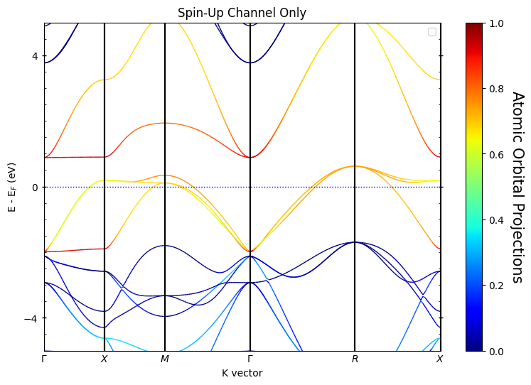
[6]:
# You can also plot specific spin channels separately
# Plot only spin-up channel
pyprocar.bandsplot(
    code='vasp',
    dirname=SPIN_POL_DATA_DIR,
    mode='parametric',
    fermi=5.3017,
    atoms=[1],
    orbitals=[4,5,6,7,8],  # d orbitals
    linestyle=('solid', 'dotted'),
    spins=[0],  # Only spin-up (index 0)
    elimit=[-5, 5],
    title='Spin-Up Channel Only',
    quiet_welcome=True
)
If you want more detailed logs, set verbose to 2 or more
____________________________________________________________________________________________________
____________________________________________________________________________________________________
____________________________________________________________________________________________________
Plotting bands in parametric mode
[6]:
(<Figure size 900x600 with 2 Axes>,
 <Axes: title={'center': 'Spin-Up Channel Only'}, xlabel='K vector', ylabel='E - E$_F$ (eV)'>)
[7]:
# Plot only spin-down channel
pyprocar.bandsplot(
    code='vasp',
    dirname=SPIN_POL_DATA_DIR,
    mode='parametric',
    fermi=5.3017,
    atoms=[1],
    orbitals=[4,5,6,7,8],  # d orbitals
    linestyle=('solid', 'dotted'),
    spins=[1],  # Only spin-down (index 1)
    elimit=[-5, 5],
    title='Spin-Down Channel Only',
    quiet_welcome=True
)
If you want more detailed logs, set verbose to 2 or more
____________________________________________________________________________________________________
____________________________________________________________________________________________________
____________________________________________________________________________________________________
Plotting bands in parametric mode

[7]:
(<Figure size 900x600 with 2 Axes>,
 <Axes: title={'center': 'Spin-Down Channel Only'}, xlabel='K vector', ylabel='E - E$_F$ (eV)'>)
3. Non-Collinear Band Structure Plotting
In non-collinear magnetic systems, the spin quantization axis is not fixed, and spin-up and spin-down states are mixed. PyProcar handles this by providing spin projections (total, sx, sy, sz).
3.1 Plain Mode - Non-Collinear Bands
First, let’s plot the basic band structure without any projections:
[8]:
# Plot non-collinear bands in plain mode
pyprocar.bandsplot(
    code='vasp',
    dirname=NON_COLLINEAR_DATA_DIR,
    mode='plain',
    fermi=5.3017,
    elimit=[-5, 5],
    title='Non-Collinear Bands (Plain Mode)',
    use_cache=True,
    quiet_welcome=True
)
If you want more detailed logs, set verbose to 2 or more
____________________________________________________________________________________________________
____________________________________________________________________________________________________
____________________________________________________________________________________________________
Plotting bands in plain mode

[8]:
(<Figure size 900x600 with 1 Axes>,
 <Axes: title={'center': 'Non-Collinear Bands (Plain Mode)'}, xlabel='K vector', ylabel='E - E$_F$ (eV)'>)
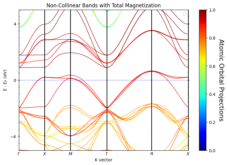
3.2 Spin Projections - Total Magnetization
In non-collinear systems, there are four spin projections. The spins argument is a list of indices that correspond to the spin channels you want to plot.
Total magnetization:
spins=[0]Sx magnetization:
spins=[1]Sy magnetization:
spins=[2]Sz magnetization:
spins=[3]
[9]:
# Plot with total magnetization projection
pyprocar.bandsplot(
    code='vasp',
    dirname=NON_COLLINEAR_DATA_DIR,
    mode='parametric',
    fermi=5.3017,
    spins=[0],
    elimit=[-5, 5],
    title='Non-Collinear Bands with Total Magnetization',
    quiet_welcome=True
)
If you want more detailed logs, set verbose to 2 or more
____________________________________________________________________________________________________
____________________________________________________________________________________________________
____________________________________________________________________________________________________
Plotting bands in parametric mode
[9]:
(<Figure size 900x600 with 2 Axes>,
 <Axes: title={'center': 'Non-Collinear Bands with Total Magnetization'}, xlabel='K vector', ylabel='E - E$_F$ (eV)'>)
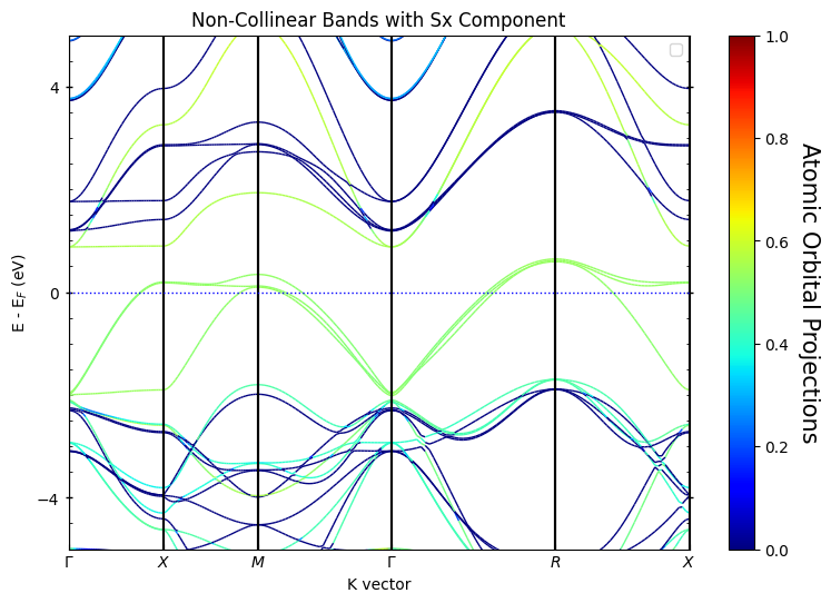
3.3 Spin Component Projections
We can also visualize the individual spin components (sx, sy, sz) to understand the spatial orientation of the magnetic moments:
[10]:
# Plot with sx component (x-direction spin)
pyprocar.bandsplot(
    code='vasp',
    dirname=NON_COLLINEAR_DATA_DIR,
    mode='parametric',
    fermi=5.3017,
    spins=[1],
    elimit=[-5, 5],
    title='Non-Collinear Bands with Sx Component',
    quiet_welcome=True
)
If you want more detailed logs, set verbose to 2 or more
____________________________________________________________________________________________________
____________________________________________________________________________________________________
____________________________________________________________________________________________________
Plotting bands in parametric mode
[10]:
(<Figure size 900x600 with 2 Axes>,
 <Axes: title={'center': 'Non-Collinear Bands with Sx Component'}, xlabel='K vector', ylabel='E - E$_F$ (eV)'>)
[11]:
# Plot with sy component (y-direction spin)
pyprocar.bandsplot(
    code='vasp',
    dirname=NON_COLLINEAR_DATA_DIR,
    mode='parametric',
    fermi=5.3017,
    spins=[2],
    elimit=[-5, 5],
    title='Non-Collinear Bands with Sy Component',
    quiet_welcome=True
)
If you want more detailed logs, set verbose to 2 or more
____________________________________________________________________________________________________
____________________________________________________________________________________________________
____________________________________________________________________________________________________
Plotting bands in parametric mode

[11]:
(<Figure size 900x600 with 2 Axes>,
 <Axes: title={'center': 'Non-Collinear Bands with Sy Component'}, xlabel='K vector', ylabel='E - E$_F$ (eV)'>)
[12]:
# Plot with sz component (z-direction spin)
pyprocar.bandsplot(
    code='vasp',
    dirname=NON_COLLINEAR_DATA_DIR,
    mode='parametric',
    fermi=5.3017,
    spins=[3],
    elimit=[-5, 5],
    title='Non-Collinear Bands with Sz Component',
    quiet_welcome=True
)
If you want more detailed logs, set verbose to 2 or more
____________________________________________________________________________________________________
____________________________________________________________________________________________________
____________________________________________________________________________________________________
Plotting bands in parametric mode

[12]:
(<Figure size 900x600 with 2 Axes>,
 <Axes: title={'center': 'Non-Collinear Bands with Sz Component'}, xlabel='K vector', ylabel='E - E$_F$ (eV)'>)
4. Summary
This tutorial demonstrated how to handle different spin configurations in PyProcar:
Key Takeaways:
Spin-Polarized Systems:
Use
spins=[0]for spin-up channel onlyUse
spins=[1]for spin-down channel onlyUse
spins=[0,1]or omit the parameter for both channelsEach spin channel is treated as a separate entity with its own bands and projections
Non-Collinear Systems:
Use
mode='parametric'to visualize spin projectionsAvailable spin projections:
'total','sx','sy','sz'Only one spin channel exists, but with 4 different spin projections
Useful for understanding magnetic anisotropy and spin orientation
Best Practices:
Always check your calculation type (spin-polarized vs non-collinear) before plotting
Use appropriate energy limits (
elimit) to focus on relevant energy rangesConsider which atoms and orbitals are most relevant for your analysis
For non-collinear systems, compare different spin components to understand the full magnetic structure