Compare Bands
Overview
The pyprocar.bandsplot() function is a powerful tool for visualizing electronic band structures. One of its key features is that it returns matplotlib Figure and Axes objects when show=False, which enables advanced plotting capabilities including comparing multiple band structures on the same plot.
What bandsplot returns
When called with show=False, bandsplot() returns:
fig: A matplotlib Figure object containing the entire plotax: A matplotlib Axes object representing the plotting area
Method for comparing band structures
To compare band structures from different codes or calculations:
First call: Use
bandsplot()withshow=Falseto generate the initial band structure and capture thefigandaxobjectsSubsequent calls: Pass the
axobject to additionalbandsplot()calls using theaxparameterFinal display: The last call should have
show=Trueto display the combined plot
This approach allows you to overlay multiple band structures from different DFT codes (like VASP and Quantum Espresso) or different calculations on the same axes for direct comparison.
Example: Comparing VASP and Quantum Espresso Band Structures
In this tutorial, we’ll compare Fe band structures calculated with both VASP and Quantum Espresso (QE) codes.
Import libraries and download example data
First, we’ll import the necessary libraries and download the example Fe band structure data for both VASP and Quantum Espresso calculations.
[1]:
# Import required libraries
from pathlib import Path
import pyprocar

CURRENT_DIR = Path(".").resolve()
print(str(CURRENT_DIR))
COMPARE_BANDS_PATH = "data/examples/bands/compare_bands"

pyprocar.download_from_hf(relpath=COMPARE_BANDS_PATH, output_path=CURRENT_DIR)
QE_DATA_DIR = CURRENT_DIR / COMPARE_BANDS_PATH / "qe"
VASP_DATA_DIR = CURRENT_DIR / COMPARE_BANDS_PATH / "vasp"
print(f"Data downloaded to: {QE_DATA_DIR}")
print(f"Data downloaded to: {VASP_DATA_DIR}")
C:\Users\lllang\Desktop\notebooks\Notebook\01 - Projects\Pyprocar\pyprocar\examples\00-band_structure
Data already exists at C:\Users\lllang\Desktop\notebooks\Notebook\01 - Projects\Pyprocar\pyprocar\examples\00-band_structure\data\examples\bands\compare_bands
Data downloaded to: C:\Users\lllang\Desktop\notebooks\Notebook\01 - Projects\Pyprocar\pyprocar\examples\00-band_structure\data\examples\bands\compare_bands\qe
Data downloaded to: C:\Users\lllang\Desktop\notebooks\Notebook\01 - Projects\Pyprocar\pyprocar\examples\00-band_structure\data\examples\bands\compare_bands\vasp
Comparing band structures
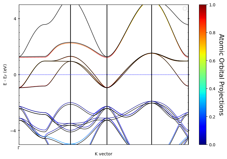
Now we’ll demonstrate the band comparison technique:
Step 1: Plot the VASP band structure with
show=Falseto capture thefigandaxobjectsStep 2: Plot the QE band structure using the same
axobject andshow=Trueto display the combined result
The VASP bands will be plotted in parametric mode (showing orbital contributions with colors) while the QE bands will be overlaid in plain mode (black lines) for clear comparison.
[2]:
print(str(VASP_DATA_DIR))
# Step 1: Plot VASP band structure and capture fig, ax objects
fig, ax = pyprocar.bandsplot(
    code="vasp",
    dirname=str(VASP_DATA_DIR),
    mode="parametric",
    fermi=5.3017,  # VASP fermi energy
    elimit=[-5, 5],
    orbitals=[4, 5, 6, 7, 8],  # d orbitals for Fe
    use_cache=False,
    show=False,  # Don't show yet, capture the axes
    quiet_welcome=True,
    verbose=3,
)

# # Step 2: Plot QE band structure on the same axes
pyprocar.bandsplot(
    code="qe",
    dirname=QE_DATA_DIR,
    mode="plain",
    fermi=12.5491,  # QE fermi energy
    elimit=[-5, 5],
    color="k",  # Black lines for QE bands
    ax=ax,  # Use the same axes from VASP plot
    show=True,  # Show the combined plot
    verbose=3,
)
C:\Users\lllang\Desktop\notebooks\Notebook\01 - Projects\Pyprocar\pyprocar\examples\00-band_structure\data\examples\bands\compare_bands\vasp
If you want more detailed logs, set verbose to 2 or more
____________________________________________________________________________________________________
____________________________________________________________________________________________________
____________________________________________________________________________________________________
[INFO] 2025-06-26 14:58:16 - pyprocar.core.ebs[1160][from_code] - Parsing EBS calculation directory: C:\Users\lllang\Desktop\notebooks\Notebook\01 - Projects\Pyprocar\pyprocar\examples\00-band_structure\data\examples\bands\compare_bands\vasp
[INFO] 2025-06-26 14:58:16 - pyprocar.io.vasp[50][__init__] - Vasp Version: 6.2.1
[DEBUG] 2025-06-26 14:58:16 - pyprocar.io.vasp[159][get_symmetry_operations] - n_spg_operations: 48
[INFO] 2025-06-26 14:58:16 - pyprocar.io.vasp[314][get_symmetry_operations] - No space group operators block found
[]
[INFO] 2025-06-26 14:58:16 - pyprocar.core.kpath[384][get_segment_indices] - Continuous indices: [39, 79, 119, 159]
[INFO] 2025-06-26 14:58:16 - pyprocar.core.kpath[385][get_segment_indices] - Discontinuity indices: []
[INFO] 2025-06-26 14:58:16 - pyprocar.core.kpath[389][get_segment_indices] - Found 5 segments
[INFO] 2025-06-26 14:58:16 - pyprocar.scripts.scriptBandsplot[150][bandsplot] - Shifting Fermi energy to zero: 5.3017
range(0, 1)
[INFO] 2025-06-26 14:58:16 - pyprocar.plotter.ebs_plot[79][__init__] - ___Initializing EBSPlot___
[DEBUG] 2025-06-26 14:58:16 - pyprocar.plotter.ebs_plot[81][__init__] - Kpath: K-Path
------
 1. $\Gamma$: (  0.00   0.00   0.00) -> X       : (  0.00   0.50   0.00)
 2. X       : (  0.00   0.50   0.00) -> M       : (  0.50   0.50   0.00)
 3. M       : (  0.50   0.50   0.00) -> $\Gamma$: (  0.00   0.00   0.00)
 4. $\Gamma$: (  0.00   0.00   0.00) -> R       : (  0.50   0.50   0.50)
 5. R       : (  0.50   0.50   0.50) -> X       : (  0.00   0.50   0.00)

Tick names:    $\Gamma$       M        $\Gamma$       R           X
Tick positions:   0           79         119         159         199
n_kpoints: 200
n_segments: 5
n_grids: [40, 40, 40, 40, 40]
discontinuity_indices: []
continuous_indices: [39, 79, 119, 159]

[DEBUG] 2025-06-26 14:58:16 - pyprocar.plotter.ebs_plot[82][__init__] - Non-collinear: False
[DEBUG] 2025-06-26 14:58:16 - pyprocar.plotter.ebs_plot[83][__init__] - Spins: range(0, 1)
[DEBUG] 2025-06-26 14:58:16 - pyprocar.plotter.ebs_plot[84][__init__] - Kdirect: True
[DEBUG] 2025-06-26 14:58:16 - pyprocar.plotter.ebs_plot[85][__init__] - Config: BandStructureConfig(plot_type=<PlotType.BAND_STRUCTURE: 'band_structure'>, custom_settings={}, modes=['plain', 'parametric', 'scatter', 'atomic', 'overlay', 'overlay_species', 'overlay_orbitals'], color='black', spin_colors=('blue', 'red'), colorbar_title='Atomic Orbital Projections', colorbar_title_size=15, colorbar_title_padding=20, colorbar_tick_labelsize=10, cmap='jet', clim=(0.0, 1.0), fermi_color='blue', fermi_linestyle='dotted', fermi_linewidth=1, grid=False, grid_axis='both', grid_color='grey', grid_linestyle='solid', grid_linewidth=1, grid_which='major', label=('$\\uparrow$', '$\\downarrow$'), legend=True, linestyle=('solid', 'dashed'), linewidth=(1.0, 1.0), marker=('o', 'v', '^', 'D'), markersize=(0.2, 0.2), opacity=(1.0, 1.0), plot_color_bar=True, savefig=None, title=None, weighted_color=True, weighted_width=False, figure_size=(9, 6), dpi=300, colorbar_tick_params={}, colorbar_label_params={}, x_label='K vector', x_label_params={}, y_label_params={}, title_params={}, major_y_tick_params={'which': 'major', 'axis': 'y', 'direction': 'inout', 'width': 1, 'length': 5, 'labelright': False, 'right': True, 'left': True}, minor_y_tick_params={'which': 'minor', 'axis': 'y', 'direction': 'in', 'left': True, 'right': True}, major_x_tick_params={'which': 'major', 'axis': 'x', 'direction': 'in'}, multiple_locator_y_major_value=None, multiple_locator_y_minor_value=None)
[DEBUG] 2025-06-26 14:58:16 - pyprocar.plotter.ebs_plot[86][__init__] - EBS:
 Electronic Band Structure
============================
Total number of kpoints   = 200
Total number of bands    = 20
Total number of atoms    = 5
Total number of orbitals = 9
Total number of spin channels = 1
Total number of spin projections = 1

Array shapes:
------------------------
projected shape = (200, 20, 1, 5, 9)
bands shape = (200, 20, 1)

Gradients:
------------------------

Hessians:
------------------------

Additional information:
Orbital Names = ['s', 'py', 'pz', 'px', 'dxy', 'dyz', 'dz2', 'dxz', 'x2-y2']
Spin Projection Names = ['Spin-up']
Non-colinear = False
Reciprocal Lattice =
 [[0.26 0.   0.  ]
 [0.   0.26 0.  ]
 [0.   0.   0.26]]
Fermi Energy = 4.5746
Has Phase = False

Structure:
------------------------
Structure =
 <pyprocar.core.structure.Structure object at 0x000001FC19F41840>

KPath:
------------------------
KPath =
 K-Path
------
 1. $\Gamma$: (  0.00   0.00   0.00) -> X       : (  0.00   0.50   0.00)
 2. X       : (  0.00   0.50   0.00) -> M       : (  0.50   0.50   0.00)
 3. M       : (  0.50   0.50   0.00) -> $\Gamma$: (  0.00   0.00   0.00)
 4. $\Gamma$: (  0.00   0.00   0.00) -> R       : (  0.50   0.50   0.50)
 5. R       : (  0.50   0.50   0.50) -> X       : (  0.00   0.50   0.00)

Tick names:    $\Gamma$       M        $\Gamma$       R           X
Tick positions:   0           79         119         159         199
n_kpoints: 200
n_segments: 5
n_grids: [40, 40, 40, 40, 40]
discontinuity_indices: []
continuous_indices: [39, 79, 119, 159]


[INFO] 2025-06-26 14:58:16 - pyprocar.plotter.ebs_plot[615][set_xticks] - ___Setting x ticks___
[DEBUG] 2025-06-26 14:58:16 - pyprocar.plotter.ebs_plot[616][set_xticks] - Setting x ticks:
        positions=[0, 79, 119, 159, 199]
        names=['$\\Gamma$', 'M', '$\\Gamma$', 'R', 'X']
        color=black
[DEBUG] 2025-06-26 14:58:16 - pyprocar.plotter.ebs_plot[626][set_xticks] - Overriding default tick_positions: [0, 79, 119, 159, 199]
[DEBUG] 2025-06-26 14:58:16 - pyprocar.plotter.ebs_plot[629][set_xticks] - Overriding default tick_names: ['$\\Gamma$', 'M', '$\\Gamma$', 'R', 'X']
[DEBUG] 2025-06-26 14:58:16 - pyprocar.plotter.ebs_plot[637][set_xticks] - tick_names: ['$\\Gamma$', 'M', '$\\Gamma$', 'R', 'X']
Plotting bands in parametric mode
[INFO] 2025-06-26 14:58:16 - pyprocar.plotter.ebs_plot[339][plot_parameteric] - ___No mask applied___
[INFO] 2025-06-26 14:58:16 - pyprocar.plotter.ebs_plot[615][set_xticks] - ___Setting x ticks___
[DEBUG] 2025-06-26 14:58:16 - pyprocar.plotter.ebs_plot[616][set_xticks] - Setting x ticks:
        positions=[0, 79, 119, 159, 199]
        names=['$\\Gamma$', 'M', '$\\Gamma$', 'R', 'X']
        color=black
[DEBUG] 2025-06-26 14:58:16 - pyprocar.plotter.ebs_plot[626][set_xticks] - Overriding default tick_positions: [0, 79, 119, 159, 199]
[DEBUG] 2025-06-26 14:58:16 - pyprocar.plotter.ebs_plot[629][set_xticks] - Overriding default tick_names: ['$\\Gamma$', 'M', '$\\Gamma$', 'R', 'X']
[DEBUG] 2025-06-26 14:58:16 - pyprocar.plotter.ebs_plot[637][set_xticks] - tick_names: ['$\\Gamma$', 'M', '$\\Gamma$', 'R', 'X']
If you want more detailed logs, set verbose to 2 or more
____________________________________________________________________________________________________
 ____        ____
|  _ \ _   _|  _ \ _ __ ___   ___ __ _ _ __
| |_) | | | | |_) | '__/ _ \ / __/ _` | '__|
|  __/| |_| |  __/| | | (_) | (_| (_| | |
|_|    \__, |_|   |_|  \___/ \___\__,_|_|
       |___/
A Python library for electronic structure pre/post-processing.

Version 6.4.6 created on Mar 6th, 2025

Please cite:
- Uthpala Herath, Pedram Tavadze, Xu He, Eric Bousquet, Sobhit Singh, Francisco Muñoz and Aldo Romero.,
  PyProcar: A Python library for electronic structure pre/post-processing.,
  Computer Physics Communications 251, 107080 (2020).

- L. Lang, P. Tavadze, A. Tellez, E. Bousquet, H. Xu, F. Muñoz, N. Vasquez, U. Herath, and A. H. Romero,
  Expanding PyProcar for new features, maintainability, and reliability.,
  Computer Physics Communications 297, 109063 (2024).

Developers:
- Francisco Muñoz
- Aldo Romero
- Sobhit Singh
- Uthpala Herath
- Pedram Tavadze
- Eric Bousquet
- Xu He
- Reese Boucher
- Logan Lang
- Freddy Farah

____________________________________________________________________________________________________

            There are additional plot options that are defined in the configuration file.
            You can change these configurations by passing the keyword argument to the function.
            To print a list of all plot options set `print_plot_opts=True`

            Here is a list modes : plain , parametric , scatter , atomic , overlay , overlay_species , overlay_orbitals

____________________________________________________________________________________________________
[INFO] 2025-06-26 14:58:16 - pyprocar.core.ebs[1160][from_code] - Parsing EBS calculation directory: C:\Users\lllang\Desktop\notebooks\Notebook\01 - Projects\Pyprocar\pyprocar\examples\00-band_structure\data\examples\bands\compare_bands\qe
[INFO] 2025-06-26 14:58:16 - pyprocar.io.qe[624][_initialize_filenames] - output_xml: C:\Users\lllang\Desktop\notebooks\Notebook\01 - Projects\Pyprocar\pyprocar\examples\00-band_structure\data\examples\bands\compare_bands\qe\out\SrVO3.xml
(151, 25, 1, 5, 9)
(151, 25, 1, 5, 9)
[]
[INFO] 2025-06-26 14:58:17 - pyprocar.core.kpath[384][get_segment_indices] - Continuous indices: []
[INFO] 2025-06-26 14:58:17 - pyprocar.core.kpath[385][get_segment_indices] - Discontinuity indices: []
[INFO] 2025-06-26 14:58:17 - pyprocar.core.kpath[389][get_segment_indices] - Found 1 segments
[INFO] 2025-06-26 14:58:17 - pyprocar.scripts.scriptBandsplot[150][bandsplot] - Shifting Fermi energy to zero: 12.5491
range(0, 1)
[INFO] 2025-06-26 14:58:17 - pyprocar.plotter.ebs_plot[79][__init__] - ___Initializing EBSPlot___
[DEBUG] 2025-06-26 14:58:17 - pyprocar.plotter.ebs_plot[81][__init__] - Kpath: K-Path
------
 1. $\Gamma$: (  0.00   0.00   0.00) -> X       : (  0.50   0.00   0.00)

Tick names:    $\Gamma$
Tick positions:   0
n_kpoints: 151
n_segments: 1
n_grids: [30, 30, 30, 30, 31]
discontinuity_indices: []
continuous_indices: []

[DEBUG] 2025-06-26 14:58:17 - pyprocar.plotter.ebs_plot[82][__init__] - Non-collinear: False
[DEBUG] 2025-06-26 14:58:17 - pyprocar.plotter.ebs_plot[83][__init__] - Spins: range(0, 1)
[DEBUG] 2025-06-26 14:58:17 - pyprocar.plotter.ebs_plot[84][__init__] - Kdirect: True
[DEBUG] 2025-06-26 14:58:17 - pyprocar.plotter.ebs_plot[85][__init__] - Config: BandStructureConfig(plot_type=<PlotType.BAND_STRUCTURE: 'band_structure'>, custom_settings={}, modes=['plain', 'parametric', 'scatter', 'atomic', 'overlay', 'overlay_species', 'overlay_orbitals'], color='k', spin_colors=('blue', 'red'), colorbar_title='Atomic Orbital Projections', colorbar_title_size=15, colorbar_title_padding=20, colorbar_tick_labelsize=10, cmap='jet', clim=(0.0, 1.0), fermi_color='blue', fermi_linestyle='dotted', fermi_linewidth=1, grid=False, grid_axis='both', grid_color='grey', grid_linestyle='solid', grid_linewidth=1, grid_which='major', label=('$\\uparrow$', '$\\downarrow$'), legend=True, linestyle=('solid', 'dashed'), linewidth=(1.0, 1.0), marker=('o', 'v', '^', 'D'), markersize=(0.2, 0.2), opacity=(1.0, 1.0), plot_color_bar=True, savefig=None, title=None, weighted_color=True, weighted_width=False, figure_size=(9, 6), dpi=300, colorbar_tick_params={}, colorbar_label_params={}, x_label='K vector', x_label_params={}, y_label_params={}, title_params={}, major_y_tick_params={'which': 'major', 'axis': 'y', 'direction': 'inout', 'width': 1, 'length': 5, 'labelright': False, 'right': True, 'left': True}, minor_y_tick_params={'which': 'minor', 'axis': 'y', 'direction': 'in', 'left': True, 'right': True}, major_x_tick_params={'which': 'major', 'axis': 'x', 'direction': 'in'}, multiple_locator_y_major_value=None, multiple_locator_y_minor_value=None)
[DEBUG] 2025-06-26 14:58:17 - pyprocar.plotter.ebs_plot[86][__init__] - EBS:
 Electronic Band Structure
============================
Total number of kpoints   = 151
Total number of bands    = 25
Total number of atoms    = 5
Total number of orbitals = 9
Total number of spin channels = 1
Total number of spin projections = 1

Array shapes:
------------------------
projected shape = (151, 25, 1, 5, 9)
projected_phase shape = (151, 25, 1, 5, 9)
bands shape = (151, 25, 1)

Gradients:
------------------------

Hessians:
------------------------

Additional information:
Orbital Names = ['s', 'py', 'pz', 'px', 'dxy', 'dyz', 'dz2', 'dxz', 'dx2']
Spin Projection Names = ['Spin-up']
Non-colinear = False
Reciprocal Lattice =
 [[1.6335 0.     0.    ]
 [0.     1.6335 0.    ]
 [0.     0.     1.6335]]
Fermi Energy = 12.5491
Has Phase = True

Structure:
------------------------
Structure =
 <pyprocar.core.structure.Structure object at 0x000001FC63E76710>

KPath:
------------------------
KPath =
 K-Path
------
 1. $\Gamma$: (  0.00   0.00   0.00) -> X       : (  0.50   0.00   0.00)

Tick names:    $\Gamma$
Tick positions:   0
n_kpoints: 151
n_segments: 1
n_grids: [30, 30, 30, 30, 31]
discontinuity_indices: []
continuous_indices: []


[INFO] 2025-06-26 14:58:17 - pyprocar.plotter.ebs_plot[615][set_xticks] - ___Setting x ticks___
[DEBUG] 2025-06-26 14:58:17 - pyprocar.plotter.ebs_plot[616][set_xticks] - Setting x ticks:
        positions=[0]
        names=['$\\Gamma$']
        color=black
[DEBUG] 2025-06-26 14:58:17 - pyprocar.plotter.ebs_plot[626][set_xticks] - Overriding default tick_positions: [0]
[DEBUG] 2025-06-26 14:58:17 - pyprocar.plotter.ebs_plot[629][set_xticks] - Overriding default tick_names: ['$\\Gamma$']
[DEBUG] 2025-06-26 14:58:17 - pyprocar.plotter.ebs_plot[637][set_xticks] - tick_names: ['$\\Gamma$']
Plotting bands in plain mode
[INFO] 2025-06-26 14:58:17 - pyprocar.plotter.ebs_plot[615][set_xticks] - ___Setting x ticks___
[DEBUG] 2025-06-26 14:58:17 - pyprocar.plotter.ebs_plot[616][set_xticks] - Setting x ticks:
        positions=[0]
        names=['$\\Gamma$']
        color=black
[DEBUG] 2025-06-26 14:58:17 - pyprocar.plotter.ebs_plot[626][set_xticks] - Overriding default tick_positions: [0]
[DEBUG] 2025-06-26 14:58:17 - pyprocar.plotter.ebs_plot[629][set_xticks] - Overriding default tick_names: ['$\\Gamma$']
[DEBUG] 2025-06-26 14:58:17 - pyprocar.plotter.ebs_plot[637][set_xticks] - tick_names: ['$\\Gamma$']
[2]:
(<Figure size 900x600 with 2 Axes>,
 <Axes: xlabel='K vector', ylabel='E - E$_F$ (eV)'>)