Getting Started: PyProcar’s fermi2D Function
This tutorial provides a comprehensive introduction to plotting 2D Fermi surfaces using PyProcar’s fermi2D function. You’ll learn about all the main arguments, visualization modes, k-space slicing, and plotting configurations.
What You’ll Learn
Core ``fermi2D`` arguments and their purposes
Different visualization modes for Fermi surface analysis
K-space plane selection and energy slicing
Spin texture visualization and parametric projections
Band-specific analysis and custom configurations
Best practices for 2D Fermi surface analysis
Prerequisites
Basic understanding of electronic band structure and Fermi surfaces
PyProcar installed in your environment
DFT calculation data with dense k-point sampling (we’ll use example data)
Overview of fermi2D Function
The fermi2D function is PyProcar’s tool for 2D Fermi surface visualization. It creates cross-sections of the Fermi surface in k-space planes. Its basic syntax is:
pyprocar.fermi2D(
    code='vasp',           # DFT code used
    dirname='.',           # Directory with calculation files
    mode='plain',          # Visualization mode
    fermi=None,           # Fermi energy
    k_z_plane=0.0,        # K_z plane for 2D slice
    # ... many other options
)
1. Setup and Data Loading
Let’s start by importing PyProcar and loading example data. We’ll use dense k-point mesh data from a DFT calculation to demonstrate 2D Fermi surface features.
[1]:
# Import required libraries
from pathlib import Path
import pyprocar

CURRENT_DIR = Path(".").resolve()
REL_PATH = "data/examples/fermi2d/non-spin-polarized"
pyprocar.download_from_hf(relpath=REL_PATH, output_path=CURRENT_DIR)
DATA_DIR = CURRENT_DIR / REL_PATH
print(f"Data downloaded to: {DATA_DIR}")
Data already exists at C:\Users\lllang\Desktop\notebooks\Notebook\01 - Projects\Pyprocar\pyprocar\examples\02-fermi2d\data\examples\fermi2d\non-spin-polarized
Data downloaded to: C:\Users\lllang\Desktop\notebooks\Notebook\01 - Projects\Pyprocar\pyprocar\examples\02-fermi2d\data\examples\fermi2d\non-spin-polarized
2. Core Arguments of fermi2D
Before exploring different modes, let’s understand the essential arguments of the fermi2D function:
Essential Arguments
Argument |
Type |
Description |
Example |
|---|---|---|---|
|
str |
DFT software used |
|
|
str |
Path to calculation files |
|
|
str |
Visualization mode |
|
|
float |
Fermi energy (eV) |
|
K-space and Energy Arguments
Argument |
Type |
Description |
Default |
|---|---|---|---|
|
float |
Energy relative to Fermi level |
|
|
float |
K_z coordinate for 2D slice |
|
|
float |
Tolerance for k_z plane selection |
|
|
float |
Shift Fermi energy |
|
Projection Arguments
Argument |
Type |
Description |
Default |
|---|---|---|---|
|
list |
Atom indices for projection |
|
|
list |
Orbital indices for projection |
|
|
list |
Spin channels |
|
|
list |
Band indices to plot |
|
|
list |
Colors for specific bands |
|
Advanced Options
Argument |
Type |
Description |
Default |
|---|---|---|---|
|
bool |
Show spin texture with arrows |
|
|
str |
Save plot filename |
|
|
list |
Rotation matrix for k-points |
|
|
list |
Translation vector for k-points |
|
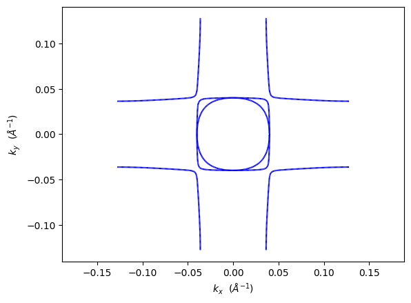
3. Basic Usage - Plain Mode
The plain mode is the simplest way to visualize 2D Fermi surfaces. It shows the Fermi surface cross-section as contour lines at the specified energy and k_z plane.
[2]:
# Basic fermi2D usage - showing essential arguments
pyprocar.fermi2D(
    code="vasp",           # Required: DFT software used
    dirname=DATA_DIR,      # Required: Directory with calculation files
    mode="plain",          # Visualization mode
    fermi=5.3017,    # Fermi energy in eV (shifts energy reference)
    energy=0.0,            # Energy relative to Fermi level (0 = Fermi surface)
    k_z_plane=0.0,         # K_z plane for 2D slice (Γ-plane)
)

print("✅ Basic 2D Fermi surface plot created with essential arguments only")
If you want more detailed logs, set verbose to 2 or more
____________________________________________________________________________________________________
 ____        ____
|  _ \ _   _|  _ \ _ __ ___   ___ __ _ _ __
| |_) | | | | |_) | '__/ _ \ / __/ _` | '__|
|  __/| |_| |  __/| | | (_) | (_| (_| | |
|_|    \__, |_|   |_|  \___/ \___\__,_|_|
       |___/
A Python library for electronic structure pre/post-processing.

Version 6.4.6 created on Mar 6th, 2025

Please cite:
- Uthpala Herath, Pedram Tavadze, Xu He, Eric Bousquet, Sobhit Singh, Francisco Muñoz and Aldo Romero.,
  PyProcar: A Python library for electronic structure pre/post-processing.,
  Computer Physics Communications 251, 107080 (2020).

- L. Lang, P. Tavadze, A. Tellez, E. Bousquet, H. Xu, F. Muñoz, N. Vasquez, U. Herath, and A. H. Romero,
  Expanding PyProcar for new features, maintainability, and reliability.,
  Computer Physics Communications 297, 109063 (2024).

Developers:
- Francisco Muñoz
- Aldo Romero
- Sobhit Singh
- Uthpala Herath
- Pedram Tavadze
- Eric Bousquet
- Xu He
- Reese Boucher
- Logan Lang
- Freddy Farah

____________________________________________________________________________________________________
### Parameters ###
dirname         : C:\Users\lllang\Desktop\notebooks\Notebook\01 - Projects\Pyprocar\pyprocar\examples\02-fermi2d\data\examples\fermi2d\non-spin-polarized
bands           : None
atoms           : None
orbitals        : None
spin comp.      : None
energy          : 0.0
rot. symmetry   : 1
origin (trasl.) : [0, 0, 0]
rotation        : [0, 0, 0, 1]
save figure     : None
spin_texture    : False
____________________________________________________________________________________________________

            There are additional plot options that are defined in a configuration file.
            You can change these configurations by passing the keyword argument to the function
            To print a list of plot options set print_plot_opts=True

            Here is a list modes : plain , plain_bands , parametric
____________________________________________________________________________________________________
WARNING: Make sure the kmesh has the correct number of kz pointswith kz=0.0 +- 0.001.
Kpoints in the kz=0.0 plane: (3721, 3)
Bands in the kz=0.0 plane: (3721, 20, 1)
Projected in the kz=0.0 plane: (3721, 20, 1, 5, 9)
Spins for projections: [0]
Atoms for projections: [0 1 2 3 4]
Orbitals for projections: [0 1 2 3 4 5 6 7 8]
Band indices near iso-surface: (bands.shape=(3721, 20)) spin-0 | bands-[16 17 18]

✅ Basic 2D Fermi surface plot created with essential arguments only
4. Visualization Modes Overview
PyProcar offers several visualization modes for different 2D Fermi surface analysis needs:
Mode |
Purpose |
Key Arguments |
Use Case |
|---|---|---|---|
|
Basic Fermi surface contours |
None extra |
Publication plots, general topology |
|
Individual band contributions |
|
Analyzing specific bands |
|
Color-coded projections |
|
Orbital/atomic character visualization |
|
Spin texture with arrows |
|
Spin-orbit coupling effects |
Mode Details
Plain: Shows clean Fermi surface contours without projections
Plain bands: Highlights specific bands with different colors
Parametric: Colors the Fermi surface by orbital/atomic character
Spin texture: Displays spin direction with arrows on the Fermi surface
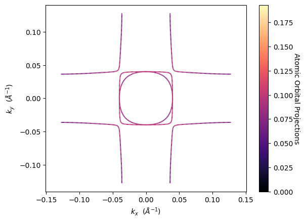
5. Parametric Mode - Projected Fermi Surface
Parametric mode shows atomic/orbital contributions through color coding on the Fermi surface. The color intensity indicates the strength of the orbital/atomic character.
Orbital Indexing Reference
s: 0
p: 1, 2, 3 (px, py, pz)
d: 4, 5, 6, 7, 8 (d orbitals)
f: 9, 10, 11, 12, 13, 14, 15 (f orbitals)
Key Features
Color mapping: Intensity shows orbital/atomic contribution strength
Multiple projections: Can combine atoms, orbitals, and spins
Quantitative analysis: Color scale provides numerical character values
[3]:
# Parametric mode requires projection arguments
pyprocar.fermi2D(
code="vasp",
dirname=DATA_DIR,
mode="parametric",
fermi=5.3017,
energy=0.0, # At Fermi level
k_z_plane=0.0, # Γ-plane slice
atoms=[2,3,4], # Project onto specific atoms (e.g., Oxygen)
orbitals=[1,2,3], # p orbitals (indices 1-3)
plot_color_bar=True, # Show color scale
)
print("🎨 Parametric mode: Color intensity shows p-orbital contribution strength")
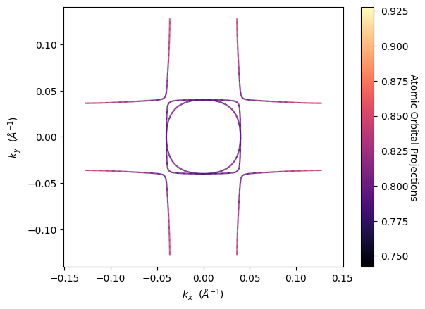
# Different orbital projection
pyprocar.fermi2D(
code="vasp",
dirname=DATA_DIR,
mode="parametric",
fermi=5.3017,
energy=0.0,
k_z_plane=0.0,
atoms=[1], # Project onto central atom (e.g., V)
orbitals=[4,5,6,7,8], # d orbitals (indices 4-8)
plot_color_bar=True,
)
print("🎨 d-orbital character visualization on Fermi surface")
If you want more detailed logs, set verbose to 2 or more
____________________________________________________________________________________________________
 ____        ____
|  _ \ _   _|  _ \ _ __ ___   ___ __ _ _ __
| |_) | | | | |_) | '__/ _ \ / __/ _` | '__|
|  __/| |_| |  __/| | | (_) | (_| (_| | |
|_|    \__, |_|   |_|  \___/ \___\__,_|_|
       |___/
A Python library for electronic structure pre/post-processing.

Version 6.4.6 created on Mar 6th, 2025

Please cite:
- Uthpala Herath, Pedram Tavadze, Xu He, Eric Bousquet, Sobhit Singh, Francisco Muñoz and Aldo Romero.,
  PyProcar: A Python library for electronic structure pre/post-processing.,
  Computer Physics Communications 251, 107080 (2020).

- L. Lang, P. Tavadze, A. Tellez, E. Bousquet, H. Xu, F. Muñoz, N. Vasquez, U. Herath, and A. H. Romero,
  Expanding PyProcar for new features, maintainability, and reliability.,
  Computer Physics Communications 297, 109063 (2024).

Developers:
- Francisco Muñoz
- Aldo Romero
- Sobhit Singh
- Uthpala Herath
- Pedram Tavadze
- Eric Bousquet
- Xu He
- Reese Boucher
- Logan Lang
- Freddy Farah

____________________________________________________________________________________________________
### Parameters ###
dirname         : C:\Users\lllang\Desktop\notebooks\Notebook\01 - Projects\Pyprocar\pyprocar\examples\02-fermi2d\data\examples\fermi2d\non-spin-polarized
bands           : None
atoms           : [2, 3, 4]
orbitals        : [1, 2, 3]
spin comp.      : None
energy          : 0.0
rot. symmetry   : 1
origin (trasl.) : [0, 0, 0]
rotation        : [0, 0, 0, 1]
save figure     : None
spin_texture    : False
____________________________________________________________________________________________________

            There are additional plot options that are defined in a configuration file.
            You can change these configurations by passing the keyword argument to the function
            To print a list of plot options set print_plot_opts=True

            Here is a list modes : plain , plain_bands , parametric
____________________________________________________________________________________________________
WARNING: Make sure the kmesh has the correct number of kz pointswith kz=0.0 +- 0.001.
Kpoints in the kz=0.0 plane: (3721, 3)
Bands in the kz=0.0 plane: (3721, 20, 1)
Projected in the kz=0.0 plane: (3721, 20, 1, 5, 9)
Spins for projections: [0]
Atoms for projections: [2, 3, 4]
Orbitals for projections: [1, 2, 3]
Band indices near iso-surface: (bands.shape=(3721, 20)) spin-0 | bands-[16 17 18]
🎨 Parametric mode: Color intensity shows p-orbital contribution strength
If you want more detailed logs, set verbose to 2 or more
____________________________________________________________________________________________________
 ____        ____
|  _ \ _   _|  _ \ _ __ ___   ___ __ _ _ __
| |_) | | | | |_) | '__/ _ \ / __/ _` | '__|
|  __/| |_| |  __/| | | (_) | (_| (_| | |
|_|    \__, |_|   |_|  \___/ \___\__,_|_|
       |___/
A Python library for electronic structure pre/post-processing.

Version 6.4.6 created on Mar 6th, 2025

Please cite:
- Uthpala Herath, Pedram Tavadze, Xu He, Eric Bousquet, Sobhit Singh, Francisco Muñoz and Aldo Romero.,
  PyProcar: A Python library for electronic structure pre/post-processing.,
  Computer Physics Communications 251, 107080 (2020).

- L. Lang, P. Tavadze, A. Tellez, E. Bousquet, H. Xu, F. Muñoz, N. Vasquez, U. Herath, and A. H. Romero,
  Expanding PyProcar for new features, maintainability, and reliability.,
  Computer Physics Communications 297, 109063 (2024).

Developers:
- Francisco Muñoz
- Aldo Romero
- Sobhit Singh
- Uthpala Herath
- Pedram Tavadze
- Eric Bousquet
- Xu He
- Reese Boucher
- Logan Lang
- Freddy Farah

____________________________________________________________________________________________________
### Parameters ###
dirname         : C:\Users\lllang\Desktop\notebooks\Notebook\01 - Projects\Pyprocar\pyprocar\examples\02-fermi2d\data\examples\fermi2d\non-spin-polarized
bands           : None
atoms           : [1]
orbitals        : [4, 5, 6, 7, 8]
spin comp.      : None
energy          : 0.0
rot. symmetry   : 1
origin (trasl.) : [0, 0, 0]
rotation        : [0, 0, 0, 1]
save figure     : None
spin_texture    : False
____________________________________________________________________________________________________

            There are additional plot options that are defined in a configuration file.
            You can change these configurations by passing the keyword argument to the function
            To print a list of plot options set print_plot_opts=True

            Here is a list modes : plain , plain_bands , parametric
____________________________________________________________________________________________________
WARNING: Make sure the kmesh has the correct number of kz pointswith kz=0.0 +- 0.001.
Kpoints in the kz=0.0 plane: (3721, 3)
Bands in the kz=0.0 plane: (3721, 20, 1)
Projected in the kz=0.0 plane: (3721, 20, 1, 5, 9)
Spins for projections: [0]
Atoms for projections: [1]
Orbitals for projections: [4, 5, 6, 7, 8]
Band indices near iso-surface: (bands.shape=(3721, 20)) spin-0 | bands-[16 17 18]
🎨 d-orbital character visualization on Fermi surface
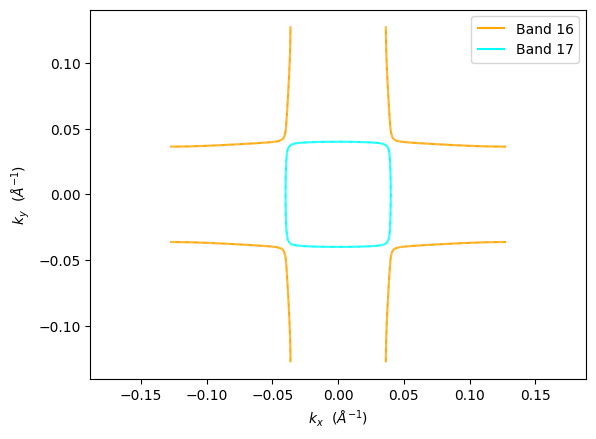
6. Plain Bands Mode - Individual Band Analysis
The plain_bands mode allows you to visualize specific bands with different colors, making it easy to identify individual band contributions to the Fermi surface.
Plain Bands Benefits
Band-specific analysis: Isolate contributions from specific bands
Color coding: Each band gets a unique color for easy identification
Topology understanding: See how different bands create Fermi surface features
Usage Tips
Use
band_indicesto specify which bands to plotUse
band_colorsto customize colors for each bandCombine with energy slicing to study band evolution
[4]:
# Plain bands mode - shows specific band contributions
pyprocar.fermi2D(
code="vasp",
dirname=DATA_DIR,
mode="plain_bands",
fermi=5.3017,
energy=0.0,
k_z_plane=0.0,
band_indices=[[16,17]], # Specify bands for each spin (if applicable)
band_colors=[['orange', 'cyan']], # Colors for each band
add_legend=True, # Show legend with band information
)
print("🎯 Plain bands mode: Shows individual band contributions with different colors")
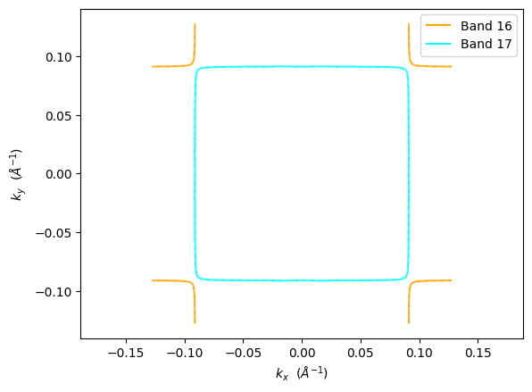
# Another example with different energy slice
pyprocar.fermi2D(
code="vasp",
dirname=DATA_DIR,
mode="plain_bands",
fermi=5.3017,
energy=1.0, # Slightly above Fermi level
k_z_plane=0.0,
band_indices=[[16,17]], # Focus on specific bands
band_colors=[['orange', 'cyan']],
add_legend=True,
)
print("🎯 Energy slice at +0.1 eV: Shows how band topology changes with energy")
If you want more detailed logs, set verbose to 2 or more
____________________________________________________________________________________________________
 ____        ____
|  _ \ _   _|  _ \ _ __ ___   ___ __ _ _ __
| |_) | | | | |_) | '__/ _ \ / __/ _` | '__|
|  __/| |_| |  __/| | | (_) | (_| (_| | |
|_|    \__, |_|   |_|  \___/ \___\__,_|_|
       |___/
A Python library for electronic structure pre/post-processing.

Version 6.4.6 created on Mar 6th, 2025

Please cite:
- Uthpala Herath, Pedram Tavadze, Xu He, Eric Bousquet, Sobhit Singh, Francisco Muñoz and Aldo Romero.,
  PyProcar: A Python library for electronic structure pre/post-processing.,
  Computer Physics Communications 251, 107080 (2020).

- L. Lang, P. Tavadze, A. Tellez, E. Bousquet, H. Xu, F. Muñoz, N. Vasquez, U. Herath, and A. H. Romero,
  Expanding PyProcar for new features, maintainability, and reliability.,
  Computer Physics Communications 297, 109063 (2024).

Developers:
- Francisco Muñoz
- Aldo Romero
- Sobhit Singh
- Uthpala Herath
- Pedram Tavadze
- Eric Bousquet
- Xu He
- Reese Boucher
- Logan Lang
- Freddy Farah

____________________________________________________________________________________________________
### Parameters ###
dirname         : C:\Users\lllang\Desktop\notebooks\Notebook\01 - Projects\Pyprocar\pyprocar\examples\02-fermi2d\data\examples\fermi2d\non-spin-polarized
bands           : [[16, 17]]
atoms           : None
orbitals        : None
spin comp.      : None
energy          : 0.0
rot. symmetry   : 1
origin (trasl.) : [0, 0, 0]
rotation        : [0, 0, 0, 1]
save figure     : None
spin_texture    : False
____________________________________________________________________________________________________

            There are additional plot options that are defined in a configuration file.
            You can change these configurations by passing the keyword argument to the function
            To print a list of plot options set print_plot_opts=True

            Here is a list modes : plain , plain_bands , parametric
____________________________________________________________________________________________________
WARNING: Make sure the kmesh has the correct number of kz pointswith kz=0.0 +- 0.001.
Kpoints in the kz=0.0 plane: (3721, 3)
Bands in the kz=0.0 plane: (3721, 20, 1)
Projected in the kz=0.0 plane: (3721, 20, 1, 5, 9)
Spins for projections: [0]
Atoms for projections: [0 1 2 3 4]
Orbitals for projections: [0 1 2 3 4 5 6 7 8]
Band indices near iso-surface: (bands.shape=(3721, 20)) spin-0 | bands-[16 17 18]
🎯 Plain bands mode: Shows individual band contributions with different colors
If you want more detailed logs, set verbose to 2 or more
____________________________________________________________________________________________________
 ____        ____
|  _ \ _   _|  _ \ _ __ ___   ___ __ _ _ __
| |_) | | | | |_) | '__/ _ \ / __/ _` | '__|
|  __/| |_| |  __/| | | (_) | (_| (_| | |
|_|    \__, |_|   |_|  \___/ \___\__,_|_|
       |___/
A Python library for electronic structure pre/post-processing.

Version 6.4.6 created on Mar 6th, 2025

Please cite:
- Uthpala Herath, Pedram Tavadze, Xu He, Eric Bousquet, Sobhit Singh, Francisco Muñoz and Aldo Romero.,
  PyProcar: A Python library for electronic structure pre/post-processing.,
  Computer Physics Communications 251, 107080 (2020).

- L. Lang, P. Tavadze, A. Tellez, E. Bousquet, H. Xu, F. Muñoz, N. Vasquez, U. Herath, and A. H. Romero,
  Expanding PyProcar for new features, maintainability, and reliability.,
  Computer Physics Communications 297, 109063 (2024).

Developers:
- Francisco Muñoz
- Aldo Romero
- Sobhit Singh
- Uthpala Herath
- Pedram Tavadze
- Eric Bousquet
- Xu He
- Reese Boucher
- Logan Lang
- Freddy Farah

____________________________________________________________________________________________________
### Parameters ###
dirname         : C:\Users\lllang\Desktop\notebooks\Notebook\01 - Projects\Pyprocar\pyprocar\examples\02-fermi2d\data\examples\fermi2d\non-spin-polarized
bands           : [[16, 17]]
atoms           : None
orbitals        : None
spin comp.      : None
energy          : 1.0
rot. symmetry   : 1
origin (trasl.) : [0, 0, 0]
rotation        : [0, 0, 0, 1]
save figure     : None
spin_texture    : False
____________________________________________________________________________________________________

            There are additional plot options that are defined in a configuration file.
            You can change these configurations by passing the keyword argument to the function
            To print a list of plot options set print_plot_opts=True

            Here is a list modes : plain , plain_bands , parametric
____________________________________________________________________________________________________
WARNING: Make sure the kmesh has the correct number of kz pointswith kz=0.0 +- 0.001.
Kpoints in the kz=0.0 plane: (3721, 3)
Bands in the kz=0.0 plane: (3721, 20, 1)
Projected in the kz=0.0 plane: (3721, 20, 1, 5, 9)
Spins for projections: [0]
Atoms for projections: [0 1 2 3 4]
Orbitals for projections: [0 1 2 3 4 5 6 7 8]
Band indices near iso-surface: (bands.shape=(3721, 20)) spin-0 | bands-[16 17 18]
🎯 Energy slice at +0.1 eV: Shows how band topology changes with energy
7. Advanced Configuration and Performance
Caching for Performance
PyProcar uses caching to speed up repeated plotting operations by storing parsed electronic band structure data:
use_cache=True   # Default: Use cached EBS data when available
use_cache=False  # Force re-parsing (useful if data changed)
Plot Customization
The fermi2D function accepts many plotting configuration options:
Option |
Description |
Example |
|---|---|---|
|
Colormap for parametric mode |
|
|
Width of Fermi surface lines |
|
|
Show k-space axis labels |
|
|
Show plot legend |
|
|
Resolution for saved figures |
|
K-point Transformations
For advanced users, k-points can be transformed:
``rotation``: Rotate k-point coordinates
[0,0,0,1](quaternion)``translate``: Translate k-points
[0,0,0]``rot_symm``: Rotational symmetry operations
1(default)
[5]:
# Advanced customization example
pyprocar.fermi2D(
    code="vasp",
    dirname=DATA_DIR,
    mode="parametric",
    fermi=5.3017,
    energy=0.0,
    k_z_plane=0.0,
    atoms=[1],                         # Central atom
    orbitals=[4,5,6,7,8],              # d orbitals

    # Appearance customizations
    cmap="plasma",                     # Custom colormap
    linewidth=1.5,                     # Thicker lines
    add_axes_labels=True,              # Show k-space labels
    add_legend=True,                   # Show legend
    plot_color_bar=True,               # Color scale

    # Save high-resolution figure
    savefig=DATA_DIR / "fermi2d_custom.png",
    dpi=300,                           # High DPI for publication

    # Performance
    use_cache=True,                    # Use cached data
    verbose=1,                         # Standard verbosity
)

print("⚙️ Advanced customization: High-quality plot with custom styling")

# Print all available plot options
pyprocar.fermi2D(
    code="vasp",
    dirname=DATA_DIR,
    mode="plain",
    fermi=5.3017,
    print_plot_opts=True,              # Print all configuration options
)

print("📋 All available plot options printed above")
If you want more detailed logs, set verbose to 2 or more
____________________________________________________________________________________________________
 ____        ____
|  _ \ _   _|  _ \ _ __ ___   ___ __ _ _ __
| |_) | | | | |_) | '__/ _ \ / __/ _` | '__|
|  __/| |_| |  __/| | | (_) | (_| (_| | |
|_|    \__, |_|   |_|  \___/ \___\__,_|_|
       |___/
A Python library for electronic structure pre/post-processing.

Version 6.4.6 created on Mar 6th, 2025

Please cite:
- Uthpala Herath, Pedram Tavadze, Xu He, Eric Bousquet, Sobhit Singh, Francisco Muñoz and Aldo Romero.,
  PyProcar: A Python library for electronic structure pre/post-processing.,
  Computer Physics Communications 251, 107080 (2020).

- L. Lang, P. Tavadze, A. Tellez, E. Bousquet, H. Xu, F. Muñoz, N. Vasquez, U. Herath, and A. H. Romero,
  Expanding PyProcar for new features, maintainability, and reliability.,
  Computer Physics Communications 297, 109063 (2024).

Developers:
- Francisco Muñoz
- Aldo Romero
- Sobhit Singh
- Uthpala Herath
- Pedram Tavadze
- Eric Bousquet
- Xu He
- Reese Boucher
- Logan Lang
- Freddy Farah

____________________________________________________________________________________________________
### Parameters ###
dirname         : C:\Users\lllang\Desktop\notebooks\Notebook\01 - Projects\Pyprocar\pyprocar\examples\02-fermi2d\data\examples\fermi2d\non-spin-polarized
bands           : None
atoms           : [1]
orbitals        : [4, 5, 6, 7, 8]
spin comp.      : None
energy          : 0.0
rot. symmetry   : 1
origin (trasl.) : [0, 0, 0]
rotation        : [0, 0, 0, 1]
save figure     : C:\Users\lllang\Desktop\notebooks\Notebook\01 - Projects\Pyprocar\pyprocar\examples\02-fermi2d\data\examples\fermi2d\non-spin-polarized\fermi2d_custom.png
spin_texture    : False
____________________________________________________________________________________________________

            There are additional plot options that are defined in a configuration file.
            You can change these configurations by passing the keyword argument to the function
            To print a list of plot options set print_plot_opts=True

            Here is a list modes : plain , plain_bands , parametric
____________________________________________________________________________________________________
WARNING: Make sure the kmesh has the correct number of kz pointswith kz=0.0 +- 0.001.
Kpoints in the kz=0.0 plane: (3721, 3)
Bands in the kz=0.0 plane: (3721, 20, 1)
Projected in the kz=0.0 plane: (3721, 20, 1, 5, 9)
Spins for projections: [0]
Atoms for projections: [1]
Orbitals for projections: [4, 5, 6, 7, 8]
Band indices near iso-surface: (bands.shape=(3721, 20)) spin-0 | bands-[16 17 18]
C:\Users\lllang\Desktop\notebooks\Notebook\01 - Projects\Pyprocar\pyprocar\pyprocar\core\fermisurface2D.py:539: UserWarning: No artists with labels found to put in legend.  Note that artists whose label start with an underscore are ignored when legend() is called with no argument.
  plt.legend()
⚙️ Advanced customization: High-quality plot with custom styling
If you want more detailed logs, set verbose to 2 or more
____________________________________________________________________________________________________
 ____        ____
|  _ \ _   _|  _ \ _ __ ___   ___ __ _ _ __
| |_) | | | | |_) | '__/ _ \ / __/ _` | '__|
|  __/| |_| |  __/| | | (_) | (_| (_| | |
|_|    \__, |_|   |_|  \___/ \___\__,_|_|
       |___/
A Python library for electronic structure pre/post-processing.

Version 6.4.6 created on Mar 6th, 2025

Please cite:
- Uthpala Herath, Pedram Tavadze, Xu He, Eric Bousquet, Sobhit Singh, Francisco Muñoz and Aldo Romero.,
  PyProcar: A Python library for electronic structure pre/post-processing.,
  Computer Physics Communications 251, 107080 (2020).

- L. Lang, P. Tavadze, A. Tellez, E. Bousquet, H. Xu, F. Muñoz, N. Vasquez, U. Herath, and A. H. Romero,
  Expanding PyProcar for new features, maintainability, and reliability.,
  Computer Physics Communications 297, 109063 (2024).

Developers:
- Francisco Muñoz
- Aldo Romero
- Sobhit Singh
- Uthpala Herath
- Pedram Tavadze
- Eric Bousquet
- Xu He
- Reese Boucher
- Logan Lang
- Freddy Farah

____________________________________________________________________________________________________
### Parameters ###
dirname         : C:\Users\lllang\Desktop\notebooks\Notebook\01 - Projects\Pyprocar\pyprocar\examples\02-fermi2d\data\examples\fermi2d\non-spin-polarized
bands           : None
atoms           : None
orbitals        : None
spin comp.      : None
energy          : None
rot. symmetry   : 1
origin (trasl.) : [0, 0, 0]
rotation        : [0, 0, 0, 1]
save figure     : None
spin_texture    : False
____________________________________________________________________________________________________

            There are additional plot options that are defined in a configuration file.
            You can change these configurations by passing the keyword argument to the function
            To print a list of plot options set print_plot_opts=True

            Here is a list modes : plain , plain_bands , parametric
add_axes_labels : {'description': 'Boolean to add axes labels', 'value': True}
add_legend : {'description': 'Boolean to add legend', 'value': False}
plot_color_bar : {'description': 'Boolean to plot the color bar', 'value': False}
cmap : {'description': 'The colormap used for the plot.', 'value': 'magma'}
clim : {'description': 'The color scale for the color bar', 'value': [None, None]}
color : {'description': 'The colors for the spin plot lines.', 'value': ['blue', 'red']}
linestyle : {'description': 'The linestyles for the spin plot lines.', 'value': ['solid', 'dashed']}
linewidth : {'description': 'The linewidth of the fermi surface', 'value': 0.2}
no_arrow : {'description': 'Boolean to use no arrows to represent the spin texture', 'value': False}
arrow_color : {'description': 'The linestyles for the spin plot lines.', 'value': None}
contour_alpha : {'description': 'The alpha value for the spin texture contour', 'value': 1.0}
arrow_density : {'description': 'The arrow density for the spin texture', 'value': 10}
arrow_size : {'description': 'The arrow size for the spin texture', 'value': 3}
spin_projection : {'description': 'The projection for the color scale for spin texture', 'value': 'z^2'}
marker : {'description': 'Controls the marker used for the spin plot', 'value': '.'}
dpi : {'description': 'The dpi value to save the image as', 'value': 'figure'}
x_label : {'description': 'The x label of the plot', 'value': '$k_{x}$  ($\\AA^{-1}$)'}
y_label : {'description': 'The x label of the plot', 'value': '$k_{y}$  ($\\AA^{-1}$)'}
____________________________________________________________________________________________________
WARNING: Make sure the kmesh has the correct number of kz pointswith kz=0.0 +- 0.001.
Kpoints in the kz=0.0 plane: (3721, 3)
Bands in the kz=0.0 plane: (3721, 20, 1)
Projected in the kz=0.0 plane: (3721, 20, 1, 5, 9)
Spins for projections: [0]
Atoms for projections: [0 1 2 3 4]
Orbitals for projections: [0 1 2 3 4 5 6 7 8]
Band indices near iso-surface: (bands.shape=(3721, 20)) spin-0 | bands-[16 17 18]
📋 All available plot options printed above
8. Best Practices and Tips
📊 Choosing the Right Mode
``’plain’``: Use for publication figures and general Fermi surface topology
``’plain_bands’``: When you need to identify specific band contributions
``’parametric’``: For analyzing orbital/atomic character on the Fermi surface
``’spin_texture’``: For systems with significant spin-orbit coupling
🎯 Key Parameters for Quality Results
Dense k-point sampling: Fermi surface plotting requires dense k-point meshes (typically 50×50×50 or higher)
Appropriate energy: Use
energy=0.0for the Fermi surface, or small values (±0.1 eV) for analysisk_z plane selection: Start with
k_z_plane=0.0(Γ-plane) for most materialsTolerance settings: Adjust
k_z_plane_tolif you have sparse k-points perpendicular to the plane
🔧 Troubleshooting Common Issues
Issue |
Solution |
|---|---|
Empty plot |
Check |
Fragmented Fermi surface |
Increase k-point density in your DFT calculation |
Missing features |
Try different |
Slow performance |
Use |
Summary
Congratulations! You’ve learned how to use PyProcar’s fermi2D function for comprehensive 2D Fermi surface analysis. Here’s what we covered:
✅ Key Concepts Mastered
Basic Usage: Essential arguments (
code,dirname,mode,fermi)Visualization Modes:
plain,plain_bands,parametric,spin_textureK-space Analysis: Plane selection with
k_z_planeandk_z_plane_tolEnergy Slicing: Constant energy surfaces with
energyparameterParametric Projections: Orbital/atomic character visualization
Advanced Configuration: Custom styling and performance optimization