Tutorial: 2D Band Structure Visualization
Introduction
Two-dimensional (2D) band structure visualization is a powerful technique for analyzing electronic properties of materials in reciprocal space. Unlike traditional 1D band structure plots that show energy dispersion along specific high-symmetry paths, 2D band structures provide a complete picture of electronic states across the entire Brillouin zone.
What are 2D Band Structures?
Physical Concept
2D band structures represent the electronic energy landscape as a function of two momentum coordinates (kₓ, kᵧ) in the Brillouin zone. This visualization technique:
Reveals complete dispersion: Shows energy variation across the entire 2D k-space
Identifies critical points: Easily spots band extrema, saddle points, and degeneracies
Visualizes topology: Reveals topological features like Dirac cones and band inversions
Enables surface analysis: Perfect for studying 2D materials and surface states
Key Applications
2D band structure plots are particularly valuable for:
2D Materials: Graphene, transition metal dichalcogenides, topological insulators
Fermi Surface Analysis: Understanding electron and hole pockets
Topological Materials: Identifying Dirac/Weyl points and topological phase transitions
Surface States: Analyzing surface band structures in thin films
Electronic Transport: Predicting conductivity and carrier mobility
Visualization Modes
PyProcar offers several visualization modes for 2D band structures:
Plain mode: Simple energy surfaces for each band
Parametric mode: Color-coded atomic/orbital projections
Property projection: Visualization of derived properties (velocity, effective mass)
Spin texture: Vector field representation of spin orientations
System Overview: Graphene as a Model System
In this tutorial, we’ll primarily use graphene as our example system because:
Simple structure: Hexagonal lattice with two carbon atoms per unit cell
Rich physics: Contains famous Dirac cones at K and K’ points
Well-understood: Extensively studied electronic structure
Excellent example: Demonstrates key concepts clearly
Graphene’s electronic structure features:
Linear dispersion: Dirac cones at K and K’ points
Zero bandgap: Semimetallic behavior
High symmetry: Hexagonal Brillouin zone
Two bands: π and π* bands from pz orbitals
Let’s begin by setting up our environment and exploring different visualization techniques.
Setting up the Environment
In this section, we’ll set up our computational environment for 2D band structure visualization. We’ll import necessary libraries and download example data for graphene calculations.
Let’s set up our environment:
[1]:
# Import required libraries
from pathlib import Path
import pyprocar
import numpy as np
import pyvista as pv

# Set up PyVista for interactive 3D plotting
# 'trame' backend enables interactive plots in Jupyter notebooks
pv.set_jupyter_backend('static')

# Setup data directories
CURRENT_DIR = Path(".").resolve()
print(f"Current working directory: {CURRENT_DIR}")

# Download the 2D band structure example data
BANDS_2D_PATH = "data/examples/bands/2d-bands"
pyprocar.download_from_hf(relpath=BANDS_2D_PATH, output_path=CURRENT_DIR)

# Define data directories for different materials
BANDS_2D_DATA_DIR = CURRENT_DIR / BANDS_2D_PATH
GRAPHENE_DATA_DIR = BANDS_2D_DATA_DIR / "graphene"
BISB_DATA_DIR = BANDS_2D_DATA_DIR / "bisb_monolayer"

print(f"2D bands data downloaded to: {BANDS_2D_DATA_DIR}")
print(f"Graphene data directory: {GRAPHENE_DATA_DIR}")
print(f"BiSb monolayer data directory: {BISB_DATA_DIR}")
Current working directory: C:\Users\lllang\Desktop\notebooks\Notebook\01 - Projects\Pyprocar\pyprocar\examples\00-band_structure
Data already exists at C:\Users\lllang\Desktop\notebooks\Notebook\01 - Projects\Pyprocar\pyprocar\examples\00-band_structure\data\examples\bands\2d-bands
2D bands data downloaded to: C:\Users\lllang\Desktop\notebooks\Notebook\01 - Projects\Pyprocar\pyprocar\examples\00-band_structure\data\examples\bands\2d-bands
Graphene data directory: C:\Users\lllang\Desktop\notebooks\Notebook\01 - Projects\Pyprocar\pyprocar\examples\00-band_structure\data\examples\bands\2d-bands\graphene
BiSb monolayer data directory: C:\Users\lllang\Desktop\notebooks\Notebook\01 - Projects\Pyprocar\pyprocar\examples\00-band_structure\data\examples\bands\2d-bands\bisb_monolayer
Example 1: Plain Mode - Basic 2D Band Structure
What is Plain Mode?
Plain mode provides the fundamental 2D band structure visualization by showing energy surfaces for selected bands across the 2D Brillouin zone. This mode:
Displays energy surfaces: Each band is represented as a 3D surface
Shows band dispersion: Reveals how energy varies with momentum
Identifies critical points: Band extrema and saddle points are clearly visible
Enables Fermi surface analysis: Can overlay Fermi level planes
Key Features for Graphene
In this example, we’ll visualize graphene’s famous π and π* bands (bands 3 and 4), which form the characteristic Dirac cones at the K and K’ points. We’ll see:
Dirac cones: Linear dispersion creating cone-shaped surfaces
Symmetry: Hexagonal Brillouin zone symmetry
Band touching: Zero bandgap at Dirac points
Extended zones: Multiple Brillouin zones for complete picture
Parameters Explanation
``bands=[3, 4]``: Focus on π and π* bands around Fermi level
``add_fermi_plane=True``: Show Fermi level as a reference plane
``extended_zone_directions``: Include neighboring Brillouin zones
``energy_lim=[-2.5, 0.8]``: Energy window around the Dirac point
Let’s create our first 2D band structure plot:
[2]:
# Initialize the handler with calculation parameters
handler = pyprocar.BandStructure2DHandler(
code="vasp", # DFT code used for calculation
dirname=GRAPHENE_DATA_DIR, # Path to calculation data
fermi=-0.795606, # Fermi energy from the calculation (in eV)
)
print("Creating plain mode 2D band structure plot...")
# Plot the 2D band structure in plain mode
handler.plot_band_structure(
mode="plain", # Basic energy surface visualization
# Fermi level visualization
add_fermi_plane=True, # Show Fermi level as reference plane
fermi_plane_size=4, # Size of Fermi plane in k-space
# Energy and k-space limits
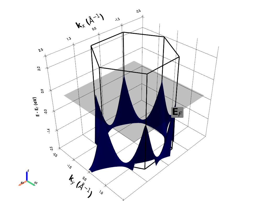
energy_lim=[-2.5, 2.0], # Energy window around Dirac point
show=True # Display the plot
)
print("\nPlot interpretation:")
print("• Two cone-shaped surfaces: π (lower) and π* (upper) bands")
print("• Dirac points: Where cones touch at K and K' points")
print("• Linear dispersion: Straight lines radiating from Dirac points")
print("• Fermi plane: Intersects exactly at the Dirac points (zero bandgap)")
print("• Hexagonal symmetry: Reflects graphene's crystal structure")
If you want more detailed logs, set verbose to 2 or more
____________________________________________________________________________________________________
 ____        ____
|  _ \ _   _|  _ \ _ __ ___   ___ __ _ _ __
| |_) | | | | |_) | '__/ _ \ / __/ _` | '__|
|  __/| |_| |  __/| | | (_) | (_| (_| | |
|_|    \__, |_|   |_|  \___/ \___\__,_|_|
       |___/
A Python library for electronic structure pre/post-processing.

Version 6.4.6 created on Mar 6th, 2025

Please cite:
- Uthpala Herath, Pedram Tavadze, Xu He, Eric Bousquet, Sobhit Singh, Francisco Muñoz and Aldo Romero.,
  PyProcar: A Python library for electronic structure pre/post-processing.,
  Computer Physics Communications 251, 107080 (2020).

- L. Lang, P. Tavadze, A. Tellez, E. Bousquet, H. Xu, F. Muñoz, N. Vasquez, U. Herath, and A. H. Romero,
  Expanding PyProcar for new features, maintainability, and reliability.,
  Computer Physics Communications 297, 109063 (2024).

Developers:
- Francisco Muñoz
- Aldo Romero
- Sobhit Singh
- Uthpala Herath
- Pedram Tavadze
- Eric Bousquet
- Xu He
- Reese Boucher
- Logan Lang
- Freddy Farah

____________________________________________________________________________________________________
Creating plain mode 2D band structure plot...
____________________________________________________________________________________________________

                There are additional plot options that are defined in a configuration file.
                You can change these configurations by passing the keyword argument to the function
                To print a list of plot options set print_plot_opts=True

                Here is a list modes : plain , parametric , spin_texture , overlay
                Here is a list of properties: bands_speed , bands_velocity , avg_inv_effective_mass

____________________________________________________________________________________________________
WARNING: Make sure the kmesh has kz points with kz=0 +- 0.0001
(3600, 10, 1)
(3600, 10, 1)
(3600, 1, 1)
(134400, 1, 1)

 Electronic Band Structure
============================
Total number of kpoints   = 134400
Total number of bands    = 1
Total number of atoms    = 2
Total number of orbitals = 9
Total number of spin channels = 1
Total number of spin projections = 1

Array shapes:
------------------------
projected shape = (134400, 1, 1, 2, 9)
bands shape = (134400, 1, 1)

Gradients:
------------------------

Hessians:
------------------------

Additional information:
Orbital Names = ['s', 'py', 'pz', 'px', 'dxy', 'dyz', 'dz2', 'dxz', 'x2-y2']
Spin Projection Names = ['Spin-up']
Non-colinear = False
Reciprocal Lattice =
 [[-0.4052 -0.234   0.    ]
 [-0.4052  0.234   0.    ]
 [ 0.      0.     -0.1151]]
Fermi Energy = -0.7955
Has Phase = False

Structure:
------------------------
Structure =
 <pyprocar.core.structure.Structure object at 0x000001C9B5D7C700>

KGrid:
------------------------
(nkx, nky, nkz) =
 [80, 80, 21]


 Electronic Band Structure
============================
Total number of kpoints   = 6400
Total number of bands    = 1
Total number of atoms    = 2
Total number of orbitals = 9
Total number of spin channels = 1
Total number of spin projections = 1

Array shapes:
------------------------
projected shape = (6400, 1, 1, 2, 9)
bands shape = (6400, 1, 1)

Gradients:
------------------------

Hessians:
------------------------

Additional information:
Orbital Names = ['s', 'py', 'pz', 'px', 'dxy', 'dyz', 'dz2', 'dxz', 'x2-y2']
Spin Projection Names = ['Spin-up']
Non-colinear = False
Reciprocal Lattice =
 [[-0.4052 -0.234   0.    ]
 [-0.4052  0.234   0.    ]
 [ 0.      0.     -0.1151]]
Fermi Energy = -0.7955
Has Phase = False

Structure:
------------------------
Structure =
 <pyprocar.core.structure.Structure object at 0x000001C9B5D7C700>

KGrid:
------------------------
(nkx, nky, nkz) =
 [80, 80, 1]

(6400, 1, 1)
c:\Users\lllang\miniconda3\envs\pyprocar\lib\site-packages\pyvista\core\filters\data_object.py:179: PyVistaDeprecationWarning: The default value of `inplace` for the filter `BandStructure2D.transform` will change in the future. Previously it defaulted to `True`, but will change to `False`. Explicitly set `inplace` to `True` or `False` to silence this warning.
  warnings.warn(msg, PyVistaDeprecationWarning)
c:\Users\lllang\miniconda3\envs\pyprocar\lib\site-packages\pyvista\core\filters\data_object.py:179: PyVistaDeprecationWarning: The default value of `inplace` for the filter `BrillouinZone2D.transform` will change in the future. Previously it defaulted to `True`, but will change to `False`. Explicitly set `inplace` to `True` or `False` to silence this warning.
  warnings.warn(msg, PyVistaDeprecationWarning)
c:\Users\lllang\miniconda3\envs\pyprocar\lib\site-packages\pyvista\core\utilities\points.py:77: UserWarning: Points is not a float type. This can cause issues when transforming or applying filters. Casting to ``np.float32``. Disable this by passing ``force_float=False``.
  warnings.warn(
To save an image of where the camera is at time when the window closes,
set the `save_2d` parameter and set `plotter_camera_pos` to the following:
 [(8.795155119873563, 8.795155119873563, 8.545155117998402),
 (0.0, 0.0, -0.25000000187516225),
 (0.0, 0.0, 1.0)]

Plot interpretation:
• Two cone-shaped surfaces: π (lower) and π* (upper) bands
• Dirac points: Where cones touch at K and K' points
• Linear dispersion: Straight lines radiating from Dirac points
• Fermi plane: Intersects exactly at the Dirac points (zero bandgap)
• Hexagonal symmetry: Reflects graphene's crystal structure
Example 2: Parametric Mode - Atomic and Orbital Projections
What is Parametric Mode?
Parametric mode enhances 2D band structure visualization by color-coding the energy surfaces according to atomic or orbital character. This reveals:
Atomic contributions: Which atoms contribute to each electronic state
Orbital character: Contribution from specific atomic orbitals (s, p, d, f)
Chemical bonding: How atomic orbitals combine to form bands
Spatial distribution: Where electronic states are localized
Graphene Orbital Analysis
For graphene, we’ll analyze the π-system formed by the pz orbitals of carbon atoms:
Two carbon atoms: Per unit cell (atoms 0 and 1)
pz orbitals: The py, px, and pz orbitals (indices 1, 2, 3)
π-bonding: Out-of-plane pz orbitals form the π and π* bands
Sublattice structure: Different contributions from A and B sublattices
Color Interpretation
In the parametric plot:
Red/warm colors: High contribution from selected atoms/orbitals
Blue/cool colors: Low contribution from selected atoms/orbitals
Color intensity: Proportional to the projection weight
Let’s visualize the orbital character of graphene’s π-bands:
[3]:
# Initialize the handler with calculation parameters
handler = pyprocar.BandStructure2DHandler(
code="vasp", # DFT code used for calculation
dirname=GRAPHENE_DATA_DIR, # Path to calculation data
fermi=-0.795606, # Fermi energy from the calculation (in eV)
)
# Parametric mode: Analyze orbital contributions to π-bands
print("Creating parametric mode visualization for graphene orbital character...")
# Define the atoms and orbitals to analyze
atoms = [0, 1] # Both carbon atoms in the unit cell
orbitals = [1, 2, 3] # px, py, pz orbitals (pz is most important for π-bands)
spins = [0] # Non-spin-polarized calculation
print(f"Analyzing atoms: {atoms} (both carbon atoms)")
print(f"Analyzing orbitals: {orbitals} (px, py, pz orbitals)")
# Plot with orbital projections
handler.plot_band_structure(
mode="parametric", # Color-code by atomic/orbital projections
atoms=atoms, # Carbon atoms to include
orbitals=orbitals, # p orbitals (especially pz)
spins=spins, # Non-spin-polarized
# Energy and k-space limits
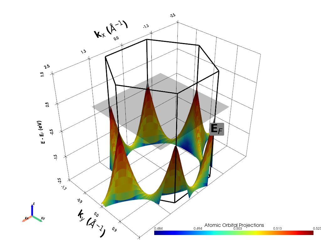
energy_lim=[-2.5, 1.5], # Energy window around Dirac point
# Visualization settings
add_fermi_plane=True, # Show Fermi level reference
fermi_plane_size=3, # Size of Fermi plane
# Save options
show=True
)
print("\nParametric plot interpretation:")
print("• Color intensity: Strength of p-orbital contribution")
print("• Red regions: High p-orbital character (especially pz)")
print("• Blue regions: Lower p-orbital contribution")
print("• π-bands: Should show strong pz character throughout")
print("• Sublattice effects: May see subtle differences between atoms 0 and 1")
If you want more detailed logs, set verbose to 2 or more
____________________________________________________________________________________________________
 ____        ____
|  _ \ _   _|  _ \ _ __ ___   ___ __ _ _ __
| |_) | | | | |_) | '__/ _ \ / __/ _` | '__|
|  __/| |_| |  __/| | | (_) | (_| (_| | |
|_|    \__, |_|   |_|  \___/ \___\__,_|_|
       |___/
A Python library for electronic structure pre/post-processing.

Version 6.4.6 created on Mar 6th, 2025

Please cite:
- Uthpala Herath, Pedram Tavadze, Xu He, Eric Bousquet, Sobhit Singh, Francisco Muñoz and Aldo Romero.,
  PyProcar: A Python library for electronic structure pre/post-processing.,
  Computer Physics Communications 251, 107080 (2020).

- L. Lang, P. Tavadze, A. Tellez, E. Bousquet, H. Xu, F. Muñoz, N. Vasquez, U. Herath, and A. H. Romero,
  Expanding PyProcar for new features, maintainability, and reliability.,
  Computer Physics Communications 297, 109063 (2024).

Developers:
- Francisco Muñoz
- Aldo Romero
- Sobhit Singh
- Uthpala Herath
- Pedram Tavadze
- Eric Bousquet
- Xu He
- Reese Boucher
- Logan Lang
- Freddy Farah

____________________________________________________________________________________________________
Creating parametric mode visualization for graphene orbital character...
Analyzing atoms: [0, 1] (both carbon atoms)
Analyzing orbitals: [1, 2, 3] (px, py, pz orbitals)
____________________________________________________________________________________________________

                There are additional plot options that are defined in a configuration file.
                You can change these configurations by passing the keyword argument to the function
                To print a list of plot options set print_plot_opts=True

                Here is a list modes : plain , parametric , spin_texture , overlay
                Here is a list of properties: bands_speed , bands_velocity , avg_inv_effective_mass

____________________________________________________________________________________________________
WARNING: Make sure the kmesh has kz points with kz=0 +- 0.0001
(3600, 10, 1)
(3600, 10, 1)
(3600, 1, 1)
(134400, 1, 1)

 Electronic Band Structure
============================
Total number of kpoints   = 134400
Total number of bands    = 1
Total number of atoms    = 2
Total number of orbitals = 9
Total number of spin channels = 1
Total number of spin projections = 1

Array shapes:
------------------------
projected shape = (134400, 1, 1, 2, 9)
bands shape = (134400, 1, 1)

Gradients:
------------------------

Hessians:
------------------------

Additional information:
Orbital Names = ['s', 'py', 'pz', 'px', 'dxy', 'dyz', 'dz2', 'dxz', 'x2-y2']
Spin Projection Names = ['Spin-up']
Non-colinear = False
Reciprocal Lattice =
 [[-0.4052 -0.234   0.    ]
 [-0.4052  0.234   0.    ]
 [ 0.      0.     -0.1151]]
Fermi Energy = -0.7955
Has Phase = False

Structure:
------------------------
Structure =
 <pyprocar.core.structure.Structure object at 0x000001C9B5D7C6D0>

KGrid:
------------------------
(nkx, nky, nkz) =
 [80, 80, 21]


 Electronic Band Structure
============================
Total number of kpoints   = 6400
Total number of bands    = 1
Total number of atoms    = 2
Total number of orbitals = 9
Total number of spin channels = 1
Total number of spin projections = 1

Array shapes:
------------------------
projected shape = (6400, 1, 1, 2, 9)
bands shape = (6400, 1, 1)

Gradients:
------------------------

Hessians:
------------------------

Additional information:
Orbital Names = ['s', 'py', 'pz', 'px', 'dxy', 'dyz', 'dz2', 'dxz', 'x2-y2']
Spin Projection Names = ['Spin-up']
Non-colinear = False
Reciprocal Lattice =
 [[-0.4052 -0.234   0.    ]
 [-0.4052  0.234   0.    ]
 [ 0.      0.     -0.1151]]
Fermi Energy = -0.7955
Has Phase = False

Structure:
------------------------
Structure =
 <pyprocar.core.structure.Structure object at 0x000001C9B5D7C6D0>

KGrid:
------------------------
(nkx, nky, nkz) =
 [80, 80, 1]

(6400, 1, 1)
c:\Users\lllang\miniconda3\envs\pyprocar\lib\site-packages\pyvista\core\filters\data_object.py:179: PyVistaDeprecationWarning: The default value of `inplace` for the filter `BandStructure2D.transform` will change in the future. Previously it defaulted to `True`, but will change to `False`. Explicitly set `inplace` to `True` or `False` to silence this warning.
  warnings.warn(msg, PyVistaDeprecationWarning)
c:\Users\lllang\miniconda3\envs\pyprocar\lib\site-packages\pyvista\core\filters\data_object.py:179: PyVistaDeprecationWarning: The default value of `inplace` for the filter `BrillouinZone2D.transform` will change in the future. Previously it defaulted to `True`, but will change to `False`. Explicitly set `inplace` to `True` or `False` to silence this warning.
  warnings.warn(msg, PyVistaDeprecationWarning)
c:\Users\lllang\miniconda3\envs\pyprocar\lib\site-packages\pyvista\core\utilities\points.py:77: UserWarning: Points is not a float type. This can cause issues when transforming or applying filters. Casting to ``np.float32``. Disable this by passing ``force_float=False``.
  warnings.warn(
To save an image of where the camera is at time when the window closes,
set the `save_2d` parameter and set `plotter_camera_pos` to the following:
 [(8.157873828404583, 8.157873828404583, 7.65787382652942),
 (0.0, 1.1102230246251565e-16, -0.5000000018751622),
 (0.0, 0.0, 1.0)]

Parametric plot interpretation:
• Color intensity: Strength of p-orbital contribution
• Red regions: High p-orbital character (especially pz)
• Blue regions: Lower p-orbital contribution
• π-bands: Should show strong pz character throughout
• Sublattice effects: May see subtle differences between atoms 0 and 1
Example 3: Property Projection Mode - Physical Properties
What is Property Projection Mode?
Property projection mode visualizes derived physical properties calculated from the electronic band structure. Instead of atomic/orbital projections, this mode shows:
Band velocity: The group velocity v = ∇_k E(k)
Effective mass: Local curvature of energy bands
Berry curvature: Topological properties of bands
Spin texture: Spin orientation in momentum space
Band Velocity Analysis
Band velocity is particularly important for transport properties:
Definition: v = (1/ℏ)∇_k E(k) - gradient of energy with respect to k
Physical meaning: Velocity of charge carriers
Units: Typically m/s or km/s for visualization
Applications: Predicting electrical and thermal conductivity
Graphene Band Velocity
For graphene, band velocity reveals:
Fermi velocity: Constant ~10⁶ m/s near Dirac points
Isotropic dispersion: Equal velocity in all directions near K points
Linear relationship: Velocity proportional to distance from Dirac point
Massless fermions: Constant velocity independent of energy
Let’s visualize the band velocity in graphene:
[4]:
# Property projection mode: Visualize band velocity
print("Creating property projection visualization for band velocity...")

# Create handler for property analysis
handler = pyprocar.BandStructure2DHandler(
    code="vasp",
    dirname=GRAPHENE_DATA_DIR,
    fermi=-0.795606,
)

print("Calculating and visualizing band velocity...")

# Plot band velocity for π and π* bands
handler.plot_band_structure(
    mode="property_projection",        # Visualize computed properties
    property_name="bands_velocity",     # Group velocity v = ∇_k E(k)

    # Energy and visualization limits
    energy_lim=[-2.5, 1.5],           # Energy window around Dirac point
    fermi_plane_size=4,                # Size of Fermi level plane

    # Color bar and scaling
    scalar_bar_position_x=0.3,        # Position of color bar

    # Reference planes
    add_fermi_plane=True,              # Show Fermi level
    show=True
)

print("\nBand velocity interpretation:")
print("• Color scale: Magnitude of group velocity |v| = |∇_k E(k)|")
print("• Near Dirac points: Constant velocity ≈ 10⁶ m/s (Fermi velocity)")
print("• Linear dispersion: Velocity increases linearly away from K points")
print("• Isotropy: Equal velocity in all directions near Dirac cones")
print("• Transport: High velocity regions contribute most to conductivity")
Creating property projection visualization for band velocity...
If you want more detailed logs, set verbose to 2 or more
____________________________________________________________________________________________________
 ____        ____
|  _ \ _   _|  _ \ _ __ ___   ___ __ _ _ __
| |_) | | | | |_) | '__/ _ \ / __/ _` | '__|
|  __/| |_| |  __/| | | (_) | (_| (_| | |
|_|    \__, |_|   |_|  \___/ \___\__,_|_|
       |___/
A Python library for electronic structure pre/post-processing.

Version 6.4.6 created on Mar 6th, 2025

Please cite:
- Uthpala Herath, Pedram Tavadze, Xu He, Eric Bousquet, Sobhit Singh, Francisco Muñoz and Aldo Romero.,
  PyProcar: A Python library for electronic structure pre/post-processing.,
  Computer Physics Communications 251, 107080 (2020).

- L. Lang, P. Tavadze, A. Tellez, E. Bousquet, H. Xu, F. Muñoz, N. Vasquez, U. Herath, and A. H. Romero,
  Expanding PyProcar for new features, maintainability, and reliability.,
  Computer Physics Communications 297, 109063 (2024).

Developers:
- Francisco Muñoz
- Aldo Romero
- Sobhit Singh
- Uthpala Herath
- Pedram Tavadze
- Eric Bousquet
- Xu He
- Reese Boucher
- Logan Lang
- Freddy Farah

____________________________________________________________________________________________________
Calculating and visualizing band velocity...
____________________________________________________________________________________________________

                There are additional plot options that are defined in a configuration file.
                You can change these configurations by passing the keyword argument to the function
                To print a list of plot options set print_plot_opts=True

                Here is a list modes : plain , parametric , spin_texture , overlay
                Here is a list of properties: bands_speed , bands_velocity , avg_inv_effective_mass

____________________________________________________________________________________________________
WARNING: Make sure the kmesh has kz points with kz=0 +- 0.0001
(3600, 10, 1)
(3600, 10, 1)
(3600, 1, 1)
(134400, 1, 1)

 Electronic Band Structure
============================
Total number of kpoints   = 134400
Total number of bands    = 1
Total number of atoms    = 2
Total number of orbitals = 9
Total number of spin channels = 1
Total number of spin projections = 1

Array shapes:
------------------------
projected shape = (134400, 1, 1, 2, 9)
bands shape = (134400, 1, 1)
bands_velocity shape = (134400, 1, 1, 3)

Gradients:
------------------------
bands shape = (134400, 1, 1, 3)

Hessians:
------------------------

Additional information:
Orbital Names = ['s', 'py', 'pz', 'px', 'dxy', 'dyz', 'dz2', 'dxz', 'x2-y2']
Spin Projection Names = ['Spin-up']
Non-colinear = False
Reciprocal Lattice =
 [[-0.4052 -0.234   0.    ]
 [-0.4052  0.234   0.    ]
 [ 0.      0.     -0.1151]]
Fermi Energy = -0.7955
Has Phase = False

Structure:
------------------------
Structure =
 <pyprocar.core.structure.Structure object at 0x000001C9B54D7DC0>

KGrid:
------------------------
(nkx, nky, nkz) =
 [80, 80, 21]


 Electronic Band Structure
============================
Total number of kpoints   = 6400
Total number of bands    = 1
Total number of atoms    = 2
Total number of orbitals = 9
Total number of spin channels = 1
Total number of spin projections = 1

Array shapes:
------------------------
projected shape = (6400, 1, 1, 2, 9)
bands_velocity shape = (6400, 1, 1, 3)
bands shape = (6400, 1, 1)

Gradients:
------------------------
bands shape = (6400, 1, 1, 3)

Hessians:
------------------------

Additional information:
Orbital Names = ['s', 'py', 'pz', 'px', 'dxy', 'dyz', 'dz2', 'dxz', 'x2-y2']
Spin Projection Names = ['Spin-up']
Non-colinear = False
Reciprocal Lattice =
 [[-0.4052 -0.234   0.    ]
 [-0.4052  0.234   0.    ]
 [ 0.      0.     -0.1151]]
Fermi Energy = -0.7955
Has Phase = False

Structure:
------------------------
Structure =
 <pyprocar.core.structure.Structure object at 0x000001C9B54D7DC0>

KGrid:
------------------------
(nkx, nky, nkz) =
 [80, 80, 1]

(6400, 1, 1)
Please select a property
---------------------------------------------------------------------------
UnboundLocalError                         Traceback (most recent call last)
Cell In[4], line 14
     11 print("Calculating and visualizing band velocity...")
     13 # Plot band velocity for π and π* bands
---> 14 handler.plot_band_structure(
     15     mode="property_projection",        # Visualize computed properties
     16     property_name="bands_velocity",     # Group velocity v = ∇_k E(k)
     17
     18     # Energy and visualization limits
     19     energy_lim=[-2.5, 1.5],           # Energy window around Dirac point
     20     fermi_plane_size=4,                # Size of Fermi level plane
     21
     22     # Color bar and scaling
     23     scalar_bar_position_x=0.3,        # Position of color bar
     24
     25     # Reference planes
     26     add_fermi_plane=True,              # Show Fermi level
     27     show=True
     28 )
     30 print("\nBand velocity interpretation:")
     31 print("• Color scale: Magnitude of group velocity |v| = |∇_k E(k)|")

File ~\Desktop\notebooks\Notebook\01 - Projects\Pyprocar\pyprocar\pyprocar\scripts\scriptBandStructure2DHandler.py:230, in BandStructure2DHandler.plot_band_structure(self, mode, bands, atoms, orbitals, spins, spin_texture, property_name, k_z_plane, k_z_plane_tol, show, k_plane_scale, render_offscreen, save_2d, save_gif, save_mp4, save_3d, print_plot_opts, **kwargs)
    219 self.data_handler.process_data(
    220     mode,
    221     bands=bands,
   (...)
    225     spin_texture=spin_texture,
    226 )
    227 band_structure_surface = self.data_handler.get_surface_data(
    228     property_name=property_name
    229 )
--> 230 visualizer = BandStructure2DVisualizer(self.data_handler, config=config)
    231 visualizer.plotter.off_screen = render_offscreen
    233 k_plane_scale_transform = np.eye(4)

File ~\Desktop\notebooks\Notebook\01 - Projects\Pyprocar\pyprocar\pyprocar\plotter\bs_2d_plot.py:267, in BandStructure2DVisualizer.__init__(self, data_handler, config)
    263 self.plotter = pv.Plotter()
    265 self.config = config
--> 267 self._setup_plotter()

File ~\Desktop\notebooks\Notebook\01 - Projects\Pyprocar\pyprocar\pyprocar\plotter\bs_2d_plot.py:700, in BandStructure2DVisualizer._setup_plotter(self)
    697     scalars = "spin_magnitude"
    698     vector_name = "spin"
--> 700 self.data_handler.text = text
    701 self.data_handler.scalars_name = scalars
    702 self.data_handler.vector_name = vector_name

UnboundLocalError: local variable 'text' referenced before assignment
Inverse Effective Mass
[7]:
# Additional analysis: Compare effective mass
print("\n" + "="*50)
print("Additional property analysis: Effective mass...")
handler_mass = pyprocar.BandStructure2DHandler(
code="vasp",
dirname=GRAPHENE_DATA_DIR,
fermi=-0.795606,
apply_symmetry=False
)
handler_mass.plot_band_structure(
mode="property_projection",
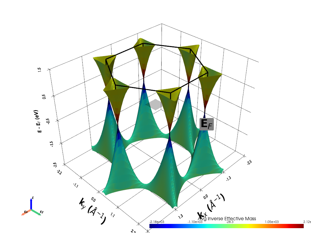
property_name="avg_inv_effective_mass", # Inverse curvature
energy_lim=[-2.5, 1.5],
add_fermi_plane=True,
show=True
)
print("• Effective mass plot created successfully")
print("• Near Dirac points: Very small effective mass (massless fermions)")
print("• Away from K points: Effective mass increases")
==================================================
Additional property analysis: Effective mass...
If you want more detailed logs, set verbose to 2 or more
____________________________________________________________________________________________________
 ____        ____
|  _ \ _   _|  _ \ _ __ ___   ___ __ _ _ __
| |_) | | | | |_) | '__/ _ \ / __/ _` | '__|
|  __/| |_| |  __/| | | (_) | (_| (_| | |
|_|    \__, |_|   |_|  \___/ \___\__,_|_|
       |___/
A Python library for electronic structure pre/post-processing.

Version 6.4.6 created on Mar 6th, 2025

Please cite:
- Uthpala Herath, Pedram Tavadze, Xu He, Eric Bousquet, Sobhit Singh, Francisco Muñoz and Aldo Romero.,
  PyProcar: A Python library for electronic structure pre/post-processing.,
  Computer Physics Communications 251, 107080 (2020).

- L. Lang, P. Tavadze, A. Tellez, E. Bousquet, H. Xu, F. Muñoz, N. Vasquez, U. Herath, and A. H. Romero,
  Expanding PyProcar for new features, maintainability, and reliability.,
  Computer Physics Communications 297, 109063 (2024).

Developers:
- Francisco Muñoz
- Aldo Romero
- Sobhit Singh
- Uthpala Herath
- Pedram Tavadze
- Eric Bousquet
- Xu He
- Reese Boucher
- Logan Lang
- Freddy Farah

____________________________________________________________________________________________________
____________________________________________________________________________________________________

                There are additional plot options that are defined in a configuration file.
                You can change these configurations by passing the keyword argument to the function
                To print a list of plot options set print_plot_opts=True

                Here is a list modes : plain , parametric , spin_texture , overlay
                Here is a list of properties: fermi_speed , fermi_velocity , harmonic_effective_mass

____________________________________________________________________________________________________
WARNING: Make sure the kmesh has kz points with kz=0 +- 0.0001
c:\Users\lllang\miniconda3\envs\pyprocar\lib\site-packages\pyvista\core\filters\data_object.py:179: PyVistaDeprecationWarning: The default value of `inplace` for the filter `BandStructure2D.transform` will change in the future. Previously it defaulted to `True`, but will change to `False`. Explicitly set `inplace` to `True` or `False` to silence this warning.
  warnings.warn(msg, PyVistaDeprecationWarning)
c:\Users\lllang\miniconda3\envs\pyprocar\lib\site-packages\pyvista\core\filters\data_object.py:179: PyVistaDeprecationWarning: The default value of `inplace` for the filter `BrillouinZone2D.transform` will change in the future. Previously it defaulted to `True`, but will change to `False`. Explicitly set `inplace` to `True` or `False` to silence this warning.
  warnings.warn(msg, PyVistaDeprecationWarning)
c:\Users\lllang\miniconda3\envs\pyprocar\lib\site-packages\pyvista\core\utilities\points.py:77: UserWarning: Points is not a float type. This can cause issues when transforming or applying filters. Casting to ``np.float32``. Disable this by passing ``force_float=False``.
  warnings.warn(
To save an image of where the camera is at time when the window closes,
set the `save_2d` parameter and set `plotter_camera_pos` to the following:
 [(8.738292852679852, 8.738292852679852, 8.238292851382866),
 (0.0, 0.0, -0.5000000012969859),
 (0.0, 0.0, 1.0)]
• Effective mass plot created successfully
• Near Dirac points: Very small effective mass (massless fermions)
• Away from K points: Effective mass increases
Example 4: Spin Texture Mode - Advanced Topological Materials
What is Spin Texture Mode?
Spin texture mode visualizes the spin orientation of electronic states across momentum space using vector fields. This advanced technique reveals:
Spin polarization: Direction and magnitude of electron spin
Topological properties: Berry curvature and Chern numbers
Rashba/Dresselhaus effects: Spin-orbit coupling signatures
Skyrmion textures: Topological spin configurations
System Change: BiSb Monolayer
For spin texture analysis, we switch to BiSb monolayer, a topological material with:
Strong spin-orbit coupling: Heavy elements (Bi, Sb) provide large SOC
Non-collinear magnetism: Spin directions vary in momentum space
Topological surface states: Protected by time-reversal symmetry
Rich spin textures: Complex spin patterns around high-symmetry points
Physical Significance
Spin texture analysis reveals:
Topological protection: How spins are locked to momentum
Transport properties: Spin-dependent conductivity
Magnetic responses: Sensitivity to external fields
Quantum phenomena: Berry phase and topological invariants
Visualization Elements
The spin texture plot shows:
Vector arrows: Direction of spin at each k-point
Color coding: Magnitude of spin components (Sx, Sy, Sz)
Surface height: Energy of electronic states
Vector density: Spatial resolution of spin sampling
Let’s explore the spin texture of BiSb monolayer:
[8]:
print("BiSb data found - proceeding with spin texture analysis...")

# Define analysis parameters
atoms = [0]                    # Focus on Bi atoms
orbitals = [4, 5, 6, 7, 8]     # d orbitals (important for SOC effects)

print(f"Analyzing atoms: {atoms} (Bi atoms)")
print(f"Analyzing orbitals: {orbitals} (d orbitals for SOC)")

# Create handler for spin texture analysis
handler = pyprocar.BandStructure2DHandler(
    code="vasp",
    dirname=BISB_DATA_DIR,     # Path to non-collinear calculation
    fermi=-1.089351,                  # Fermi energy for BiSb
    apply_symmetry=False,           # Keep all k-points for texture
)

print("Creating spin texture visualization...")

# Plot spin texture
handler.plot_band_structure(
    mode="spin_texture",            # Activate spin texture mode
    spin_texture=True,              # Enable vector field display

    # Atomic and orbital selection
    atoms=atoms,                    # Bi atoms
    orbitals=orbitals,              # d orbitals
    spins=[3],                      # Sz component

    # Energy and spatial limits
    energy_lim=[-2, 2],             # Wide energy window
    fermi_plane_size=2,             # Fermi level reference
    add_fermi_plane=True,           # Show Fermi level

    # Visualization settings
    scalar_bar_position_x=0.3,      # Color bar position
    fermi_text_position=[0, 0.5, 0], # Fermi level label position

    # Save options
    show=True
)

print("\nSpin texture interpretation:")
print("• Vector arrows: Local spin direction at each k-point")
print("• Arrow length: Magnitude of spin polarization")
print("• Color coding: Spin component values (Sx, Sy, Sz)")
print("• Swirling patterns: Topological spin textures")
print("• Singularities: Points where spin direction is undefined")
print("• Rashba effect: Spin locked perpendicular to momentum")

print("\nTopological significance:")
print("• Spin-momentum locking: Spins tied to crystal momentum")
print("• Berry curvature: Related to topological charge")
print("• Protected states: Robust against perturbations")
print("• Transport: Spin-dependent conductivity patterns")
BiSb data found - proceeding with spin texture analysis...
Analyzing atoms: [0] (Bi atoms)
Analyzing orbitals: [4, 5, 6, 7, 8] (d orbitals for SOC)
If you want more detailed logs, set verbose to 2 or more
____________________________________________________________________________________________________
 ____        ____
|  _ \ _   _|  _ \ _ __ ___   ___ __ _ _ __
| |_) | | | | |_) | '__/ _ \ / __/ _` | '__|
|  __/| |_| |  __/| | | (_) | (_| (_| | |
|_|    \__, |_|   |_|  \___/ \___\__,_|_|
       |___/
A Python library for electronic structure pre/post-processing.

Version 6.4.6 created on Mar 6th, 2025

Please cite:
- Uthpala Herath, Pedram Tavadze, Xu He, Eric Bousquet, Sobhit Singh, Francisco Muñoz and Aldo Romero.,
  PyProcar: A Python library for electronic structure pre/post-processing.,
  Computer Physics Communications 251, 107080 (2020).

- L. Lang, P. Tavadze, A. Tellez, E. Bousquet, H. Xu, F. Muñoz, N. Vasquez, U. Herath, and A. H. Romero,
  Expanding PyProcar for new features, maintainability, and reliability.,
  Computer Physics Communications 297, 109063 (2024).

Developers:
- Francisco Muñoz
- Aldo Romero
- Sobhit Singh
- Uthpala Herath
- Pedram Tavadze
- Eric Bousquet
- Xu He
- Reese Boucher
- Logan Lang
- Freddy Farah

____________________________________________________________________________________________________
Creating spin texture visualization...
____________________________________________________________________________________________________

                There are additional plot options that are defined in a configuration file.
                You can change these configurations by passing the keyword argument to the function
                To print a list of plot options set print_plot_opts=True

                Here is a list modes : plain , parametric , spin_texture , overlay
                Here is a list of properties: fermi_speed , fermi_velocity , harmonic_effective_mass

____________________________________________________________________________________________________
WARNING: Make sure the kmesh has kz points with kz=0 +- 0.0001
c:\Users\lllang\miniconda3\envs\pyprocar\lib\site-packages\pyvista\core\filters\data_object.py:179: PyVistaDeprecationWarning: The default value of `inplace` for the filter `BandStructure2D.transform` will change in the future. Previously it defaulted to `True`, but will change to `False`. Explicitly set `inplace` to `True` or `False` to silence this warning.
  warnings.warn(msg, PyVistaDeprecationWarning)
c:\Users\lllang\miniconda3\envs\pyprocar\lib\site-packages\pyvista\core\filters\data_object.py:179: PyVistaDeprecationWarning: The default value of `inplace` for the filter `BrillouinZone2D.transform` will change in the future. Previously it defaulted to `True`, but will change to `False`. Explicitly set `inplace` to `True` or `False` to silence this warning.
  warnings.warn(msg, PyVistaDeprecationWarning)

To save an image of where the camera is at time when the window closes,
set the `save_2d` parameter and set `plotter_camera_pos` to the following:
 [(6.435664180437791, 6.4356642996470805, 6.431334141413438),
 (-1.1920928955078125e-07, 0.0, -0.004330158233642578),
 (0.0, 0.0, 1.0)]

Spin texture interpretation:
• Vector arrows: Local spin direction at each k-point
• Arrow length: Magnitude of spin polarization
• Color coding: Spin component values (Sx, Sy, Sz)
• Swirling patterns: Topological spin textures
• Singularities: Points where spin direction is undefined
• Rashba effect: Spin locked perpendicular to momentum

Topological significance:
• Spin-momentum locking: Spins tied to crystal momentum
• Berry curvature: Related to topological charge
• Protected states: Robust against perturbations
• Transport: Spin-dependent conductivity patterns
Summary and Advanced Techniques
What We Learned
This tutorial demonstrated the power of 2D band structure visualization using PyProcar. We explored four distinct visualization modes:
1. Plain Mode
Purpose: Basic energy surface visualization
Key insight: Revealed graphene’s Dirac cones and linear dispersion
Applications: Fundamental band structure analysis, Fermi surface identification
2. Parametric Mode
Purpose: Atomic and orbital character analysis
Key insight: Confirmed π-character of graphene bands from pz orbitals
Applications: Chemical bonding analysis, orbital hybridization studies
3. Property Projection Mode
Purpose: Physical property visualization
Key insight: Showed constant Fermi velocity in graphene’s linear bands
Applications: Transport property prediction, effective mass analysis
4. Spin Texture Mode
Purpose: Advanced topological analysis
Key insight: Demonstrated spin-momentum locking in topological materials
Applications: Topological characterization, spintronics research
PyProcar 2D Workflow Summary
# Standard 2D band structure workflow
handler = pyprocar.BandStructure2DHandler(
    code="vasp",
    dirname="path/to/data",
    fermi=fermi_energy,
    apply_symmetry=False    # Keep full BZ for 2D plots
)

handler.plot_band_structure(
    mode="plain",           # or "parametric", "property_projection", "spin_texture"
    bands=[list],           # Specific bands of interest
    energy_lim=[emin, emax], # Energy window
    save_3d="output.html",  # Interactive 3D
    save_2d="output.png",   # 2D slice
    show=True
)