Getting Started: PyProcar’s bandsplot Function

This tutorial provides a comprehensive introduction to plotting band structures using PyProcar’s bandsplot function. You’ll learn about all the main arguments, visualization modes, caching options, and plotting configurations.

What You’ll Learn

• Core ``bandsplot`` arguments and their purposes

• Different visualization modes for band structure analysis

• Caching functionality to speed up repeated plotting

• Plotting configurations for customizing appearance

• Best practices for different analysis scenarios

Prerequisites

• Basic understanding of electronic band structures

• PyProcar installed in your environment

• VASP calculation data (we’ll use SrVO3 example data)

Overview of bandsplot Function

The bandsplot function is PyProcar’s main tool for band structure visualization. Its basic syntax is:

pyprocar.bandsplot(
    code='vasp',           # DFT code used
    dirname='.',           # Directory with calculation files
    mode='plain',          # Visualization mode
    fermi=None,           # Fermi energy
    # ... many other options
)

1. Setup and Data Loading

Let’s start by importing PyProcar and loading example data. We’ll use SrVO3 band structure data from a VASP calculation to demonstrate all the features.

# Import required libraries
from pathlib import Path
import pyprocar

CURRENT_DIR = Path(".").resolve()
REL_PATH = "data/examples/bands/non-spin-polarized"
pyprocar.download_from_hf(relpath=REL_PATH, output_path=CURRENT_DIR)
DATA_DIR = CURRENT_DIR / REL_PATH
print(f"Data downloaded to: {DATA_DIR}")

c:\Users\lllang\miniconda3\envs\pyprocar\lib\site-packages\tqdm\auto.py:21: TqdmWarning: IProgress not found. Please update jupyter and ipywidgets. See https://ipywidgets.readthedocs.io/en/stable/user_install.html
  from .autonotebook import tqdm as notebook_tqdm

Uncompressing examples subdirectories...
Uncompressing examples\00-band_structure\non-spin-polarized.zip...
Data downloaded to: C:\Users\lllang\Desktop\notebooks\Notebook\01 - Projects\Pyprocar\pyprocar\examples\00-band_structure\data\examples\00-band_structure\non-spin-polarized

2. Core Arguments of bandsplot

Before exploring different modes, let’s understand the essential arguments of the bandsplot function:

Essential Arguments

Argument	Type	Description	Example
code	str	DFT software used	'vasp', 'qe', 'abinit'
dirname	str	Path to calculation files	'.', '/path/to/data'
mode	str	Visualization mode	'plain', 'parametric', 'overlay'
fermi	float	Fermi energy (eV)	5.599

Optional Arguments

Argument	Type	Description	Default
atoms	list	Atom indices for projection	None
orbitals	list	Orbital indices for projection	None
spins	list	Spin channels	None
savefig	str	Save plot filename	None
title	str	Plot title	None

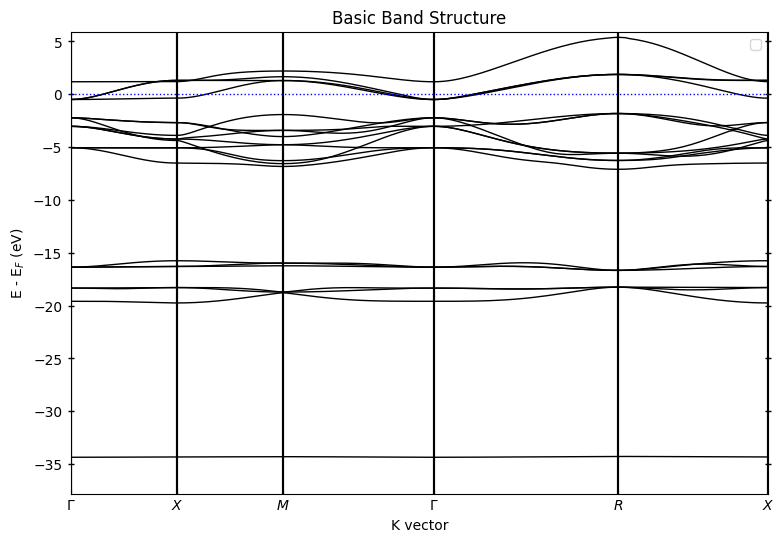
3. Basic Usage - Plain Mode

The plain mode is the simplest way to visualize band structures. It shows clean band lines without projections.

# Basic bandsplot usage - showing essential arguments
pyprocar.bandsplot(
    code="vasp",           # Required: DFT software used
    dirname=DATA_DIR,      # Required: Directory with calculation files
    mode="plain",          # Visualization mode
    fermi=5.3017,        # Fermi energy in eV (shifts energy reference)
    title="Basic Band Structure"  # Optional: add a title
)

print("✅ Basic plot created with essential arguments only")

If you want more detailed logs, set verbose to 2 or more
____________________________________________________________________________________________________
 ____        ____
|  _ \ _   _|  _ \ _ __ ___   ___ __ _ _ __
| |_) | | | | |_) | '__/ _ \ / __/ _` | '__|
|  __/| |_| |  __/| | | (_) | (_| (_| | |
|_|    \__, |_|   |_|  \___/ \___\__,_|_|
       |___/
A Python library for electronic structure pre/post-processing.

Version 6.4.6 created on Mar 6th, 2025

Please cite:
- Uthpala Herath, Pedram Tavadze, Xu He, Eric Bousquet, Sobhit Singh, Francisco Muñoz and Aldo Romero.,
  PyProcar: A Python library for electronic structure pre/post-processing.,
  Computer Physics Communications 251, 107080 (2020).

- L. Lang, P. Tavadze, A. Tellez, E. Bousquet, H. Xu, F. Muñoz, N. Vasquez, U. Herath, and A. H. Romero,
  Expanding PyProcar for new features, maintainability, and reliability.,
  Computer Physics Communications 297, 109063 (2024).

Developers:
- Francisco Muñoz
- Aldo Romero
- Sobhit Singh
- Uthpala Herath
- Pedram Tavadze
- Eric Bousquet
- Xu He
- Reese Boucher
- Logan Lang
- Freddy Farah

____________________________________________________________________________________________________

            There are additional plot options that are defined in the configuration file.
            You can change these configurations by passing the keyword argument to the function.
            To print a list of all plot options set `print_plot_opts=True`

            Here is a list modes : plain , parametric , scatter , atomic , overlay , overlay_species , overlay_orbitals

____________________________________________________________________________________________________
Plotting bands in plain mode

✅ Basic plot created with essential arguments only

4. Visualization Modes Overview

PyProcar offers several visualization modes for different analysis needs:

Mode	Purpose	Key Arguments	Use Case
'plain'	Basic band plot	None extra	Publication plots, general overview
'parametric'	Projected bands	atoms, orbitals, spins	Analyzing specific contributions
'scatter'	Point-based plot	atoms, orbitals, spins	Discrete contributions
'overlay'	Custom overlays	items	Comparing multiple projections
'overlay_species'	Compare elements	orbitals, spins	Multi-element systems
'overlay_orbitals'	Compare orbitals	atoms, spins	Orbital analysis

5. Scatter/Parametric Mode - Projected Band Structures

Parametric mode shows atomic/orbital contributions through band thickness or color intensity.

Orbital Indexing Reference

• s: 0

• p: 1, 2, 3 (px, py, pz)

• d: 4, 5, 6, 7, 8 (d orbitals)

• f: 9, 10, 11, 12, 13, 14, 15 (f orbitals)

# Parametric mode requires projection arguments
pyprocar.bandsplot(
    code="vasp",
    dirname=DATA_DIR,
    mode="parametric",
    fermi=5.3017,
    atoms=[2,3,4],                # Project onto all the Oxygen atoms
    orbitals=[1,2,3], # p orbitals (indices 1-3)
    title="SrVO$_3$ - O p-orbital contributions",
    quiet_welcome=True
)


print("📊 Parametric mode: Band thickness/color shows d-orbital contribution strength")


pyprocar.bandsplot(
    code="vasp",
    dirname=DATA_DIR,
    mode="scatter",
    fermi=5.3017,
    atoms=[1],                # Project onto all the Oxygen atoms
    orbitals=[4,5,6,7,8], # p orbitals (indices 1-3)
    title="SrVO$_3$ - V d-orbital contributions",
    quiet_welcome=True
)

If you want more detailed logs, set verbose to 2 or more
____________________________________________________________________________________________________
____________________________________________________________________________________________________
____________________________________________________________________________________________________
Plotting bands in parametric mode

📊 Parametric mode: Band thickness/color shows d-orbital contribution strength
If you want more detailed logs, set verbose to 2 or more
____________________________________________________________________________________________________
____________________________________________________________________________________________________
____________________________________________________________________________________________________
Plotting bands in scatter mode

(<Figure size 900x600 with 2 Axes>,
 <Axes: title={'center': 'SrVO$_3$ - V d-orbital contributions'}, xlabel='K vector', ylabel='E - E$_F$ (eV)'>)

6. The Cache Argument - Speeding Up Repeated Plots

PyProcar by default caches parsed data to speed up repeated plotting with different parameters. This cached data is stored in pkl files. This is especially useful when experimenting with different visualization options or when the system is very large.

How Caching Works

1. First run: PyProcar reads and parses all calculation files. The data is then stored in pkl files within the calculation directory.

2. Subsequent runs: PyProcar loads cached data (much faster)

3. Cache location: Stored in the calculation directory

# First plot - data will be parsed and cached
print("First run:")
pyprocar.bandsplot(
    code="vasp",
    dirname=DATA_DIR,
    mode="plain",
    fermi=5.3017,
    cache=False,  # Enable caching (default is True)
    title="Cached Data - Plain Mode",
    quiet_welcome=True
)

First run:
If you want more detailed logs, set verbose to 2 or more
____________________________________________________________________________________________________
____________________________________________________________________________________________________
____________________________________________________________________________________________________
Plotting bands in plain mode

(<Figure size 900x600 with 1 Axes>,
 <Axes: title={'center': 'Cached Data - Plain Mode'}, xlabel='K vector', ylabel='E - E$_F$ (eV)'>)

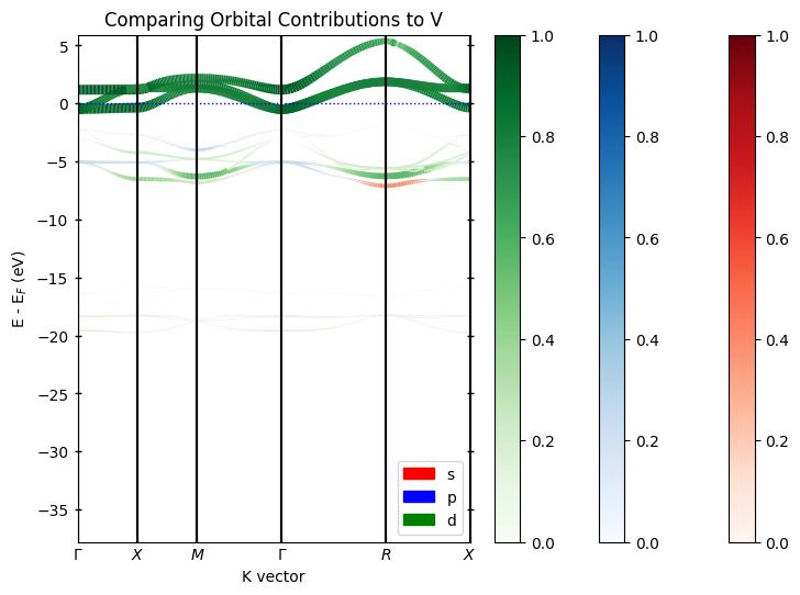
7. Overlay Modes - Comparing Multiple Contributions

Overlay modes allow you to compare different contributions on the same plot. Each contribution gets a different color and appears in the legend.

Available Overlay Modes

• ``overlay_species``: Compare different atomic species

• ``overlay_orbitals``: Compare different orbital types

• ``overlay``: Custom user-defined comparisons

# overlay_orbitals: Compare different orbital types
pyprocar.bandsplot(
    code="vasp",
    dirname=DATA_DIR,
    mode="overlay_species",
    fermi=5.3017,
    orbitals=[1,2,3],
    title="Comparing Species Contributions to p-orbitals",
    quiet_welcome=True
)

# overlay_orbitals: Compare different orbital types
pyprocar.bandsplot(
    code="vasp",
    dirname=DATA_DIR,
    mode="overlay_orbitals",
    fermi=5.3017,
    atoms=[1],  # V atom
    title="Comparing Orbital Contributions to V",
    quiet_welcome=True
)

# overlay: Custom comparisons using the items argument
items = {
    "V": [1,2,3],        # s orbital
    "O": [1,2,3],   # p orbitals
    "V": [4,5,6,7,8] # d orbitals
}

pyprocar.bandsplot(
    code="vasp",
    dirname=DATA_DIR,
    mode="overlay",
    fermi=5.3017,
    items=items,  # Custom orbital groupings
    title="Custom Orbital Comparison",
    quiet_welcome=True
)

print("🎨 Overlay modes: Each contribution gets a unique color in the legend")

If you want more detailed logs, set verbose to 2 or more
____________________________________________________________________________________________________
____________________________________________________________________________________________________
____________________________________________________________________________________________________
Plotting bands in overlay species mode

If you want more detailed logs, set verbose to 2 or more
____________________________________________________________________________________________________
____________________________________________________________________________________________________
____________________________________________________________________________________________________
Plotting bands in overlay orbitals mode

If you want more detailed logs, set verbose to 2 or more
____________________________________________________________________________________________________
____________________________________________________________________________________________________
____________________________________________________________________________________________________
Plotting bands in overlay mode

🎨 Overlay modes: Each contribution gets a unique color in the legend

8. Plotting Configurations - Customizing Appearance

PyProcar provides extensive options to customize plot appearance through various configuration arguments.

Key Configuration Arguments

Category	Arguments	Description
Labels	title, xlabel, ylabel	Plot titles and axis labels
Energy	fermi, elimit	Energy reference and plot range
Colors	cmap, clim	Colormap and color limits
Size	markersize, linewidth	Point and line sizes
Output	savefig, dpi	Save options

pyprocar.bandsplot(
    code="vasp",
    dirname=DATA_DIR,
    mode="plain",
    fermi=5.3017,
    print_plot_opts=True,
    quiet_welcome=True
)

If you want more detailed logs, set verbose to 2 or more
____________________________________________________________________________________________________
____________________________________________________________________________________________________
plot_type : PlotType.BAND_STRUCTURE
custom_settings : {}
modes : ['plain', 'parametric', 'scatter', 'atomic', 'overlay', 'overlay_species', 'overlay_orbitals']
color : black
spin_colors : ('blue', 'red')
colorbar_title : Atomic Orbital Projections
colorbar_title_size : 15
colorbar_title_padding : 20
colorbar_tick_labelsize : 10
cmap : jet
clim : (0.0, 1.0)
fermi_color : blue
fermi_linestyle : dotted
fermi_linewidth : 1
grid : False
grid_axis : both
grid_color : grey
grid_linestyle : solid
grid_linewidth : 1
grid_which : major
label : ('$\\uparrow$', '$\\downarrow$')
legend : True
linestyle : ('solid', 'dashed')
linewidth : (1.0, 1.0)
marker : ('o', 'v', '^', 'D')
markersize : (0.2, 0.2)
opacity : (1.0, 1.0)
plot_color_bar : True
savefig : None
title : None
weighted_color : True
weighted_width : False
figure_size : (9, 6)
dpi : 300
colorbar_tick_params : {}
colorbar_label_params : {}
x_label : K vector
x_label_params : {}
y_label_params : {}
title_params : {}
major_y_tick_params : {'which': 'major', 'axis': 'y', 'direction': 'inout', 'width': 1, 'length': 5, 'labelright': False, 'right': True, 'left': True}
minor_y_tick_params : {'which': 'minor', 'axis': 'y', 'direction': 'in', 'left': True, 'right': True}
major_x_tick_params : {'which': 'major', 'axis': 'x', 'direction': 'in'}
multiple_locator_y_major_value : None
multiple_locator_y_minor_value : None
____________________________________________________________________________________________________
Plotting bands in plain mode

(<Figure size 900x600 with 1 Axes>,
 <Axes: xlabel='K vector', ylabel='E - E$_F$ (eV)'>)

# Example 1: Customizing energy range and labels
pyprocar.bandsplot(
    code="vasp",
    dirname=DATA_DIR,
    mode="plain",
    fermi=5.3017,
    elimit=[-3, 3],  # Energy range: -3 to +3 eV around Fermi
    title="Customized Band Structure",
    minor_y_tick_params={'direction': 'inout', 'width': 1, 'length': 5, 'labelright': False, 'right': True, 'left': True},
    multiple_locator_y_minor_value=0.5,
    xlabel="Wave Vector",
    ylabel="Energy - E_F (eV)",
    quiet_welcome=True
)

# Example 2: Customizing colors and markers for parametric plot
pyprocar.bandsplot(
    code="vasp",
    dirname=DATA_DIR,
    mode="parametric",
    fermi=5.3017,
    atoms=[1],
    orbitals=[4,5,6,7,8],
    cmap="plasma",     # Different colormap
    clim=[0, 0.5],     # Color scale limits
    markersize=2,      # Smaller markers
    title="Custom Colors and Markers",
    quiet_welcome=True
)

print("🎨 Configuration options allow full customization of plot appearance")

If you want more detailed logs, set verbose to 2 or more
____________________________________________________________________________________________________
____________________________________________________________________________________________________
____________________________________________________________________________________________________
Plotting bands in plain mode

If you want more detailed logs, set verbose to 2 or more
____________________________________________________________________________________________________
____________________________________________________________________________________________________
____________________________________________________________________________________________________
Plotting bands in parametric mode

🎨 Configuration options allow full customization of plot appearance

9. Saving and Output Options

PyProcar provides several options for saving plots and controlling output quality.

Save Options

# Saving plots with different formats and quality
pyprocar.bandsplot(
    code="vasp",
    dirname=DATA_DIR,
    mode="plain",
    fermi=5.3017,
    title="Publication Quality Band Structure",
    savefig=DATA_DIR / "band_structure.png",  # Save as PNG
    elimit=[-4, 4]
)

# Alternative: Save as vector format (better for publications)
pyprocar.bandsplot(
    code="vasp",
    dirname=DATA_DIR,
    mode="parametric",
    fermi=5.3017,
    atoms=[0],
    orbitals=[4,5,6,7,8],
    spins=[0],
    savefig=DATA_DIR / "band_structure_parametric.pdf",  # Vector format
    dpi=300,
    title="Vector Format Export"
)

print("💾 Plots saved as:")
print("   - band_structure.png (300 DPI raster)")
print("   - band_structure_parametric.pdf (vector format)")

If you want more detailed logs, set verbose to 2 or more
____________________________________________________________________________________________________
 ____        ____
|  _ \ _   _|  _ \ _ __ ___   ___ __ _ _ __
| |_) | | | | |_) | '__/ _ \ / __/ _` | '__|
|  __/| |_| |  __/| | | (_) | (_| (_| | |
|_|    \__, |_|   |_|  \___/ \___\__,_|_|
       |___/
A Python library for electronic structure pre/post-processing.

Version 6.4.6 created on Mar 6th, 2025

Please cite:
- Uthpala Herath, Pedram Tavadze, Xu He, Eric Bousquet, Sobhit Singh, Francisco Muñoz and Aldo Romero.,
  PyProcar: A Python library for electronic structure pre/post-processing.,
  Computer Physics Communications 251, 107080 (2020).

- L. Lang, P. Tavadze, A. Tellez, E. Bousquet, H. Xu, F. Muñoz, N. Vasquez, U. Herath, and A. H. Romero,
  Expanding PyProcar for new features, maintainability, and reliability.,
  Computer Physics Communications 297, 109063 (2024).

Developers:
- Francisco Muñoz
- Aldo Romero
- Sobhit Singh
- Uthpala Herath
- Pedram Tavadze
- Eric Bousquet
- Xu He
- Reese Boucher
- Logan Lang
- Freddy Farah

____________________________________________________________________________________________________

            There are additional plot options that are defined in the configuration file.
            You can change these configurations by passing the keyword argument to the function.
            To print a list of all plot options set `print_plot_opts=True`

            Here is a list modes : plain , parametric , scatter , atomic , overlay , overlay_species , overlay_orbitals

____________________________________________________________________________________________________
Plotting bands in plain mode

<Figure size 900x600 with 0 Axes>

If you want more detailed logs, set verbose to 2 or more
____________________________________________________________________________________________________
 ____        ____
|  _ \ _   _|  _ \ _ __ ___   ___ __ _ _ __
| |_) | | | | |_) | '__/ _ \ / __/ _` | '__|
|  __/| |_| |  __/| | | (_) | (_| (_| | |
|_|    \__, |_|   |_|  \___/ \___\__,_|_|
       |___/
A Python library for electronic structure pre/post-processing.

Version 6.4.6 created on Mar 6th, 2025

Please cite:
- Uthpala Herath, Pedram Tavadze, Xu He, Eric Bousquet, Sobhit Singh, Francisco Muñoz and Aldo Romero.,
  PyProcar: A Python library for electronic structure pre/post-processing.,
  Computer Physics Communications 251, 107080 (2020).

- L. Lang, P. Tavadze, A. Tellez, E. Bousquet, H. Xu, F. Muñoz, N. Vasquez, U. Herath, and A. H. Romero,
  Expanding PyProcar for new features, maintainability, and reliability.,
  Computer Physics Communications 297, 109063 (2024).

Developers:
- Francisco Muñoz
- Aldo Romero
- Sobhit Singh
- Uthpala Herath
- Pedram Tavadze
- Eric Bousquet
- Xu He
- Reese Boucher
- Logan Lang
- Freddy Farah

____________________________________________________________________________________________________

            There are additional plot options that are defined in the configuration file.
            You can change these configurations by passing the keyword argument to the function.
            To print a list of all plot options set `print_plot_opts=True`

            Here is a list modes : plain , parametric , scatter , atomic , overlay , overlay_species , overlay_orbitals

____________________________________________________________________________________________________
Plotting bands in parametric mode

<Figure size 900x600 with 0 Axes>

💾 Plots saved as:
   - band_structure.png (300 DPI raster)
   - band_structure_parametric.pdf (vector format)

Summary: Mastering bandsplot

🎉 Congratulations! You’ve learned the complete bandsplot function including:

Core Concepts Covered

1. Essential arguments: code, dirname, mode, fermi

2. Visualization modes: plain, parametric, overlay_*

3. Caching: Speed up repeated plotting with cache=True

4. Configurations: Customize appearance with colors, labels, limits

5. Output options: Save high-quality plots for publications

💡 Key Takeaways

Concept	Key Points
Arguments	Start with code, dirname, mode, fermi
Modes	Choose based on analysis goal
Caching	Always use cache=True for efficiency
Configuration	Customize with title, elimit, cmap, etc.
Best Practices	Use orbital names, meaningful titles

🚀 Quick Reference

# Basic usage
pyprocar.bandsplot(code='vasp', dirname='.', mode='plain', fermi=E_F)

# With projections
pyprocar.bandsplot(code='vasp', dirname='.', mode='parametric',
                  fermi=E_F, atoms=[0], orbitals=[4,5,6,7,8], spins=[0])

# Custom overlays
pyprocar.bandsplot(code='vasp', dirname='.', mode='overlay',
                  fermi=E_F, items={'d-orbitals': ['d']})