De Haas-van Alphen Frequencies from Fermi Surfaces
Understanding Quantum Oscillations in Metals
The de Haas-van Alphen (dHvA) effect is a quantum mechanical phenomenon where the magnetization of a metal oscillates as a function of applied magnetic field. This effect provides one of the most precise methods to map Fermi surfaces experimentally.
What are de Haas-van Alphen frequencies?
When a magnetic field is applied to a metal, electrons in the Fermi surface undergo cyclotron motion. The dHvA frequencies correspond to the different cyclotron orbits that electrons can take on the Fermi surface. Each frequency is directly related to an extremal cross-sectional area of the Fermi surface when cut by planes perpendicular to the magnetic field direction.
The Physics Behind the Formula
The dHvA frequency F is given by the Onsager relation:
Where:
\(F\) is the dHvA frequency (in Tesla or Gauss)
\(\hbar = 1.0546 \times 10^{-27}\) erg·s (reduced Planck constant)
\(e = 4.768 \times 10^{-10}\) statcoulombs (elementary charge in CGS)
\(A_{extremal}\) is the extremal cross-sectional area of the Fermi surface (in cm⁻²)
Why Extremal Areas Matter
Not all cross-sections contribute to dHvA oscillations! Only extremal cross-sectional areas (maxima, minima, or saddle points) produce observable oscillations. This is because:
Stationary phase condition: Only orbits where the cross-sectional area is stationary with respect to the position of the cutting plane survive the quantum interference
Constructive interference: Electrons in extremal orbits maintain phase coherence, leading to observable oscillations
Tutorial Objectives
In this tutorial, we will:
Calculate the Fermi surface of gold (Au) using DFT data
Find extremal cross-sectional areas along different crystallographic directions
Convert these areas to dHvA frequencies using the Onsager relation
Compare our theoretical results with experimental measurements
Experimental Reference
We compare our results with the classic experimental study: “The Fermi surfaces of copper, silver and gold. I. The de Haas-Van alphen effect” by Shoenberg (1962), Proc. Roy. Soc. A, doi: 10.1098/rsta.1962.0011
Data Setup
The calculation files for this tutorial will be downloaded automatically in the next cell.
Import Libraries and Download Data
We’ll use PyProcar to analyze the Fermi surface of gold from DFT calculations. The example data contains a VASP calculation with the necessary files to construct the 3D Fermi surface.
[14]:
# Import required libraries
from pathlib import Path
import pyprocar
import pyvista as pv
pv.set_jupyter_backend('static')

CURRENT_DIR = Path(".").resolve()
REL_PATH = "data/examples/fermi3d/van-alphen"
pyprocar.download_from_hf(relpath=REL_PATH, output_path=CURRENT_DIR)
DATA_DIR = CURRENT_DIR / REL_PATH
print(f"Data downloaded to: {DATA_DIR}")
Data already exists at C:\Users\lllang\Desktop\notebooks\Notebook\01 - Projects\Pyprocar\pyprocar\examples\04-fermi3d\data\examples\fermi3d\van-alphen
Data downloaded to: C:\Users\lllang\Desktop\notebooks\Notebook\01 - Projects\Pyprocar\pyprocar\examples\04-fermi3d\data\examples\fermi3d\van-alphen
[15]:
# Create FermiHandler object - this loads and processes the DFT data
fermiHandler = pyprocar.FermiHandler(
    code="vasp",           # DFT software used (VASP in this case)
    dirname=DATA_DIR,      # Directory containing VASPRUN.xml, EIGENVAL, etc.
    apply_symmetry=True,   # Use crystal symmetry to reduce computational cost
    use_cache=False,       # Don't use cached data for this tutorial
    fermi=8.5642,          # Fermi energy from DFT calculation (eV)
    verbose=0              # Minimal output for cleaner tutorial
)

print("✅ FermiHandler object created successfully!")
print("   - Electronic band structure loaded from VASP files")
print("   - Fermi surface ready for cross-sectional analysis")
print(f"   - Using Fermi energy: {fermiHandler.ebs.efermi:.4f} eV")
print(f"   - k-point mesh: {fermiHandler.ebs.nkpoints} k-points")
print(f"   - Number of bands: {fermiHandler.ebs.nbands}")
 ____        ____
|  _ \ _   _|  _ \ _ __ ___   ___ __ _ _ __
| |_) | | | | |_) | '__/ _ \ / __/ _` | '__|
|  __/| |_| |  __/| | | (_) | (_| (_| | |
|_|    \__, |_|   |_|  \___/ \___\__,_|_|
       |___/
A Python library for electronic structure pre/post-processing.

Version 6.4.6 created on Mar 6th, 2025

Please cite:
- Uthpala Herath, Pedram Tavadze, Xu He, Eric Bousquet, Sobhit Singh, Francisco Muñoz and Aldo Romero.,
  PyProcar: A Python library for electronic structure pre/post-processing.,
  Computer Physics Communications 251, 107080 (2020).

- L. Lang, P. Tavadze, A. Tellez, E. Bousquet, H. Xu, F. Muñoz, N. Vasquez, U. Herath, and A. H. Romero,
  Expanding PyProcar for new features, maintainability, and reliability.,
  Computer Physics Communications 297, 109063 (2024).

Developers:
- Francisco Muñoz
- Aldo Romero
- Sobhit Singh
- Uthpala Herath
- Pedram Tavadze
- Eric Bousquet
- Xu He
- Reese Boucher
- Logan Lang
- Freddy Farah

Parsing KPOINTS file: C:\Users\lllang\Desktop\notebooks\Notebook\01 - Projects\Pyprocar\pyprocar\examples\04-fermi3d\data\examples\fermi3d\van-alphen\KPOINTS
[INFO] 2025-06-15 09:11:33 - pyprocar.scripts.scriptFermiHandler[104][__init__] - Detected symmetry operations ((48, 3, 3)). Applying to ebs to get full BZ
[DEBUG] 2025-06-15 09:11:33 - pyprocar.core.ebs[1213][ibz2fbz] - Number of kpoints in ibz: 120
[DEBUG] 2025-06-15 09:11:33 - pyprocar.core.ebs[1214][ibz2fbz] - Number of rotations: 48
[DEBUG] 2025-06-15 09:11:33 - pyprocar.core.ebs[1270][ibz2fbz] - Number of kpoints in full BZ: 3375
✅ FermiHandler object created successfully!
   - Electronic band structure loaded from VASP files
   - Fermi surface ready for cross-sectional analysis
   - Using Fermi energy: 8.5642 eV
   - k-point mesh: 3375 k-points
   - Number of bands: 20
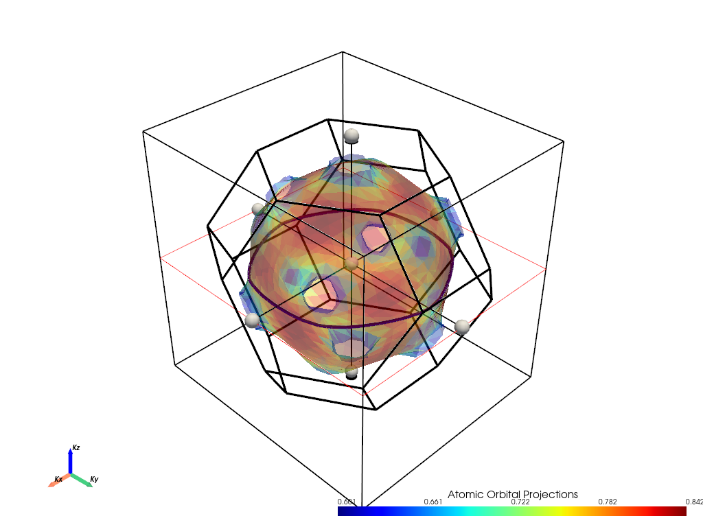
Finding Extremal Cross-Sections for dHvA Frequencies
Understanding Gold’s Fermi Surface
Gold has an FCC crystal structure with a nearly spherical Fermi surface (often called the “belly” orbit). However, there are also “neck” orbits that connect different sheets of the Fermi surface. For dHvA measurements, we need to find the extremal cross-sectional areas.
1. Maximum Cross-Sectional Area along [001] Direction
First, let’s examine cross-sections perpendicular to the crystallographic [001] direction (z-axis). We expect to find the maximum cross-sectional area at the center of the Brillouin zone, corresponding to the “belly” orbit.
Why these parameters?
bands=[5]: We focus on band 5, which contains the Fermi surface of interestslice_normal=(0, 0, 1): Cut perpendicular to the z-axis ([001] direction)slice_origin=(0, 0, 0): Start at the Γ-point (center of Brillouin zone)mode="parametric": Show orbital projections for better visualizationsurface_opacity=0.40: Semi-transparent surface to see internal structure
[16]:
# Interactive cross-section analysis
# The box widget allows you to move the cutting plane to find extremal areas
fermiHandler.plot_fermi_cross_section_box_widget(
    bands=[5],                    # Band 5 contains the Fermi surface
    slice_normal=(0, 0, 1),      # Cut perpendicular to [001] direction
    slice_origin=(0, 0, 0),      # Start at Γ-point (k=0,0,0)
    surface_opacity=0.40,        # Semi-transparent for better visualization
    mode="parametric",           # Show orbital character projections
    show=True,                   # Display the interactive plot
)
____________________________________________________________________________________________________

                There are additional plot options that are defined in a configuration file.
                You can change these configurations by passing the keyword argument to the function
                To print a list of plot options set print_plot_opts=True

                Here is a list modes : plain , parametric , spin_texture , overlay
                Here is a list of properties: fermi_speed , fermi_velocity , harmonic_effective_mass
____________________________________________________________________________________________________
[INFO] 2025-06-15 09:11:33 - pyprocar.plotter.fermi3d_plot[301][process_data] - ___Processing data fermi surface___
[INFO] 2025-06-15 09:11:33 - pyprocar.plotter.fermi3d_plot[115][_determine_bands_near_fermi] - ___Determining bands near fermi___
[INFO] 2025-06-15 09:11:33 - pyprocar.plotter.fermi3d_plot[132][_determine_bands_near_fermi] - Bands Near Fermi : [5]
[INFO] 2025-06-15 09:11:33 - pyprocar.plotter.fermi3d_plot[133][_determine_bands_near_fermi] - ____End of bands near fermi processing___
[INFO] 2025-06-15 09:11:33 - pyprocar.plotter.fermi3d_plot[60][_determine_spin_projections] - ___Determining spin projections___
[INFO] 2025-06-15 09:11:33 - pyprocar.plotter.fermi3d_plot[61][_determine_spin_projections] - Initial spins: None
[INFO] 2025-06-15 09:11:33 - pyprocar.plotter.fermi3d_plot[77][_determine_spin_projections] - Final spins: [0].
[INFO] 2025-06-15 09:11:33 - pyprocar.plotter.fermi3d_plot[78][_determine_spin_projections] - Final spin_pol: [0]. This is intented
[INFO] 2025-06-15 09:11:33 - pyprocar.plotter.fermi3d_plot[79][_determine_spin_projections] - ____End of spin projections processing___
[INFO] 2025-06-15 09:11:33 - pyprocar.plotter.fermi3d_plot[137][_process_spd] - ___Processing spd___
[INFO] 2025-06-15 09:11:33 - pyprocar.plotter.fermi3d_plot[83][_process_data_for_parametric_mode] - ___Processing data for parametric mode___
[INFO] 2025-06-15 09:11:33 - pyprocar.plotter.fermi3d_plot[106][_process_data_for_parametric_mode] - Orbitals considered: [0 1 2 3 4 5 6 7 8]
[INFO] 2025-06-15 09:11:33 - pyprocar.plotter.fermi3d_plot[107][_process_data_for_parametric_mode] - Atoms considered: [0]
[INFO] 2025-06-15 09:11:33 - pyprocar.plotter.fermi3d_plot[108][_process_data_for_parametric_mode] - Final spins: [0]
[INFO] 2025-06-15 09:11:33 - pyprocar.plotter.fermi3d_plot[109][_process_data_for_parametric_mode] - spd after summing over the projections shape: (3375, 1, 1)
[INFO] 2025-06-15 09:11:33 - pyprocar.plotter.fermi3d_plot[110][_process_data_for_parametric_mode] - First kpoint and bands: [0.506]
[INFO] 2025-06-15 09:11:33 - pyprocar.plotter.fermi3d_plot[111][_process_data_for_parametric_mode] - ____End of parametric mode processing___
[DEBUG] 2025-06-15 09:11:33 - pyprocar.plotter.fermi3d_plot[146][_process_spd] - spd after summing over the projections shape: (3375, 1, 1)
[INFO] 2025-06-15 09:11:33 - pyprocar.plotter.fermi3d_plot[147][_process_spd] - ____End of spd processing___
[INFO] 2025-06-15 09:11:33 - pyprocar.plotter.fermi3d_plot[153][_process_spd_spin_texture] - ___Processing spd_spin_texture___
[INFO] 2025-06-15 09:11:33 - pyprocar.plotter.fermi3d_plot[181][_process_spd_spin_texture] - ____End of spd_spin_texture processing___
[INFO] 2025-06-15 09:11:33 - pyprocar.plotter.fermi3d_plot[325][get_surface_data] - ____ Getting Fermi Surface Data ____
[INFO] 2025-06-15 09:11:33 - pyprocar.plotter.fermi3d_plot[185][_initialize_properties] - ___Initializing properties___
[DEBUG] 2025-06-15 09:11:33 - pyprocar.plotter.fermi3d_plot[337][get_surface_data] - Bands shape for spin 0: (3375, 1)
[INFO] 2025-06-15 09:11:33 - pyprocar.core.fermisurface3D[72][__init__] - ___Initializing the FermiSurface3D object___
[DEBUG] 2025-06-15 09:11:33 - pyprocar.core.fermisurface3D[76][__init__] - ebs.bands shape: (3375, 1)
[DEBUG] 2025-06-15 09:11:33 - pyprocar.core.fermisurface3D[83][__init__] - ebs.kpoints shape: (3375, 3)
[DEBUG] 2025-06-15 09:11:33 - pyprocar.core.fermisurface3D[84][__init__] - First 3 ebs.kpoints: [[0.4667 0.4667 0.4667]
 [0.4667 0.4667 0.4   ]
 [0.4667 0.4667 0.3333]]
[INFO] 2025-06-15 09:11:33 - pyprocar.core.fermisurface3D[92][__init__] - Iso-value used to find isosurfaces: 8.5642
[INFO] 2025-06-15 09:11:33 - pyprocar.core.fermisurface3D[93][__init__] - Interpolation factor: 1
[INFO] 2025-06-15 09:11:33 - pyprocar.core.fermisurface3D[94][__init__] - Projection accuracy: high
[INFO] 2025-06-15 09:11:33 - pyprocar.core.fermisurface3D[95][__init__] - Supercell used to calculate the FermiSurface3D: [1 1 1]
[INFO] 2025-06-15 09:11:33 - pyprocar.core.fermisurface3D[96][__init__] - Maximum distance to keep points from isosurface centers: 0.3
[INFO] 2025-06-15 09:11:33 - pyprocar.core.brillouin_zone[72][__init__] - ___Initializing BrillouinZone object___
[INFO] 2025-06-15 09:11:33 - pyprocar.core.brillouin_zone[143][wigner_seitz] - ___Calculating Wigner Seitz cell___
[DEBUG] 2025-06-15 09:11:33 - pyprocar.core.brillouin_zone[87][__init__] - BrillouinZone faces: 14
[DEBUG] 2025-06-15 09:11:33 - pyprocar.core.brillouin_zone[88][__init__] - BrillouinZone verts: (48, 3)
[INFO] 2025-06-15 09:11:33 - pyprocar.core.brillouin_zone[170][_fix_normals_direction] - ___Fixing normals direction___
[INFO] 2025-06-15 09:11:33 - pyprocar.core.fermisurface3D[123][_generate_isosurfaces] - ____Generating isosurfaces for each band___
[DEBUG] 2025-06-15 09:11:33 - pyprocar.core.fermisurface3D[127][_generate_isosurfaces] - ebs.bands_mesh shape: (15, 15, 15, 1)
[INFO] 2025-06-15 09:11:33 - pyprocar.core.isosurface[85][__init__] - ____ Initializing Isosurface ____
[DEBUG] 2025-06-15 09:11:33 - pyprocar.core.isosurface[86][__init__] - XYZ shape: (3375, 3)
[DEBUG] 2025-06-15 09:11:33 - pyprocar.core.isosurface[87][__init__] - isovalue: 8.5642
[DEBUG] 2025-06-15 09:11:33 - pyprocar.core.isosurface[91][__init__] - V_matrix shape: (15, 15, 15)
[DEBUG] 2025-06-15 09:11:33 - pyprocar.core.isosurface[92][__init__] - algorithm: lewiner
[DEBUG] 2025-06-15 09:11:33 - pyprocar.core.isosurface[93][__init__] - interpolation_factor: 1
[DEBUG] 2025-06-15 09:11:33 - pyprocar.core.isosurface[94][__init__] - padding: [1 1 1]
[DEBUG] 2025-06-15 09:11:33 - pyprocar.core.isosurface[96][__init__] - transform_matrix shape: (3, 3)
[DEBUG] 2025-06-15 09:11:33 - pyprocar.core.isosurface[98][__init__] - boundaries:
 BrillouinZone (0x2d943a46680)
  N Cells:    14
  N Points:   48
  N Strips:   0
  X Bounds:   -2.543e-01, 2.543e-01
  Y Bounds:   -4.404e-01, 4.404e-01
  Z Bounds:   -4.844e-01, 4.844e-01
  N Arrays:   0
[DEBUG] 2025-06-15 09:11:33 - pyprocar.core.isosurface[231][surface_boundaries] - ____ Getting surface boundaries ____
[DEBUG] 2025-06-15 09:11:33 - pyprocar.core.isosurface[443][_get_isosurface] - ____ Applying marching cubes ____
[DEBUG] 2025-06-15 09:11:33 - pyprocar.core.isosurface[444][_get_isosurface] - eigen_matrix shape: (29, 29, 29)
[DEBUG] 2025-06-15 09:11:33 - pyprocar.core.isosurface[445][_get_isosurface] - isovalue: 8.5642
[DEBUG] 2025-06-15 09:11:33 - pyprocar.core.isosurface[387][_process_isosurface] - ____ Processing isosurface ____
[DEBUG] 2025-06-15 09:11:33 - pyprocar.core.isosurface[327][_apply_transform_matrix] - ____ Applying transform matrix ____
[DEBUG] 2025-06-15 09:11:33 - pyprocar.core.isosurface[356][_apply_boundaries] - ____ Applying boundaries ____
[DEBUG] 2025-06-15 09:11:33 - pyprocar.core.fermisurface3D[147][_generate_isosurfaces] - Found isosurface with 1232 points
[DEBUG] 2025-06-15 09:11:33 - pyprocar.core.fermisurface3D[161][_generate_isosurfaces] - self.ebs.bands shape: (3375, 1) after removing bands with no isosurfaces
[INFO] 2025-06-15 09:11:33 - pyprocar.core.fermisurface3D[164][_generate_isosurfaces] - Band Isosurface index map: {0: 0}
[INFO] 2025-06-15 09:11:33 - pyprocar.core.fermisurface3D[168][_combine_isosurfaces] - ____Combining isosurfaces___
[INFO] 2025-06-15 09:11:33 - pyprocar.core.fermisurface3D[180][_combine_isosurfaces] - Number of points on isosurface 0 isosurface: 1232
[INFO] 2025-06-15 09:11:33 - pyprocar.core.fermisurface3D[116][__init__] - ___End of initialization FermiSurface3D object___
[WARNING] 2025-06-15 09:11:33 - pyprocar.core.fermisurface3D[431][is_empty_mesh] - No Fermi surface found. Skipping surface addition.
[INFO] 2025-06-15 09:11:33 - pyprocar.core.fermisurface3D[522][project_atomic_projections] - ____Starting Projecting atomic projections___
[DEBUG] 2025-06-15 09:11:33 - pyprocar.core.fermisurface3D[523][project_atomic_projections] - spd shape at this point: (3375, 1)
[INFO] 2025-06-15 09:11:33 - pyprocar.core.fermisurface3D[532][project_atomic_projections] - scalars_array shape after the creation of the array from the spd: (3375, 1)
[INFO] 2025-06-15 09:11:33 - pyprocar.core.fermisurface3D[449][_project_color] - ____Starting Projecting atomic projections___
[DEBUG] 2025-06-15 09:11:33 - pyprocar.core.fermisurface3D[472][_project_color] - Number of points before projecting inside the Brillouin zone: 23625
[DEBUG] 2025-06-15 09:11:33 - pyprocar.core.fermisurface3D[482][_project_color] - Number of points after determining which points are near isosurface centers: 16407
[DEBUG] 2025-06-15 09:11:33 - pyprocar.core.fermisurface3D[485][_project_color] - Number of scalars after determining which points are near isosurface centers: 16407
[INFO] 2025-06-15 09:11:35 - pyprocar.core.fermisurface3D[515][_project_color] - ___End of projecting scalars___
[INFO] 2025-06-15 09:11:35 - pyprocar.plotter.fermi3d_plot[255][_merge_fermi_surfaces] - ____ Merging Fermi Surfaces of different spins ____
[INFO] 2025-06-15 09:11:35 - pyprocar.plotter.fermi3d_plot[406][get_surface_data] - ____ Retrieived Fermi Surface Data ____
Bands being used if bands=None:
[INFO] 2025-06-15 09:11:36 - pyprocar.plotter.fermi3d_plot[446][add_surface] - ____Adding Surface to Plotter____
[WARNING] 2025-06-15 09:11:36 - pyprocar.core.fermisurface3D[431][is_empty_mesh] - No Fermi surface found. Skipping surface addition.
[INFO] 2025-06-15 09:11:36 - pyprocar.plotter.fermi3d_plot[860][_setup_band_colors] - ____ Setting up Band Colors ____
[INFO] 2025-06-15 09:11:36 - pyprocar.plotter.fermi3d_plot[873][_generate_band_colors] - ____ Generating Band Colors ____
[DEBUG] 2025-06-15 09:11:36 - pyprocar.plotter.fermi3d_plot[883][_generate_band_colors] - Band Colors: [[0.  0.  0.5 1. ]]
[DEBUG] 2025-06-15 09:11:36 - pyprocar.plotter.fermi3d_plot[884][_generate_band_colors] - Band Colors shape: (1, 4)
[INFO] 2025-06-15 09:11:36 - pyprocar.plotter.fermi3d_plot[885][_generate_band_colors] - ____ Finished Generating Band Colors ____
[INFO] 2025-06-15 09:11:36 - pyprocar.plotter.fermi3d_plot[889][_apply_fermi_surface_band_colors] - ____ Applying Band Colors ____
[INFO] 2025-06-15 09:11:36 - pyprocar.plotter.fermi3d_plot[912][_apply_fermi_surface_band_colors] - ____ Finished Applying Band Colors ____
[INFO] 2025-06-15 09:11:36 - pyprocar.plotter.fermi3d_plot[869][_setup_band_colors] - ____ Finished Setting up Band Colors ____
[DEBUG] 2025-06-15 09:11:36 - pyprocar.plotter.fermi3d_plot[478][add_surface] - Adding surface with scalars: scalars
[DEBUG] 2025-06-15 09:11:36 - pyprocar.plotter.fermi3d_plot[481][add_surface] - surface:
 FermiSurface3D (0x2d92dc34160)
  N Cells:    2252
  N Points:   1232
  N Strips:   0
  X Bounds:   -1.884e-01, 1.884e-01
  Y Bounds:   -2.081e-01, 2.081e-01
  Z Bounds:   -2.076e-01, 2.076e-01
  N Arrays:   4
[DEBUG] 2025-06-15 09:11:36 - pyprocar.plotter.fermi3d_plot[482][add_surface] - surface.point_data:
 pyvista DataSetAttributes
Association     : POINT
Active Scalars  : band_index
Active Vectors  : None
Active Texture  : None
Active Normals  : None
Contains arrays :
    band_index              int32      (1232,)              SCALARS
    bands                   float64    (1232, 4)
[DEBUG] 2025-06-15 09:11:36 - pyprocar.plotter.fermi3d_plot[483][add_surface] - surface.cell_data:
 ['band_index', 'scalars']
[INFO] 2025-06-15 09:11:36 - pyprocar.plotter.fermi3d_plot[800][show] - Showing plot
Analysis of Maximum Cross-Section
In the interactive plot above, move the cutting plane to find the maximum cross-sectional area. This corresponds to the “belly” orbit of gold’s Fermi surface.
Expected Results:
Cross-sectional area: \(A_{max} = 4.1586\) Å\(^{-2}\) = \(4.1586 \times 10^{16}\) cm\(^{-2}\)
This represents the largest cyclotron orbit electrons can take in the [001] direction
Physical Interpretation:
This orbit encompasses the main body of the Fermi surface
Electrons in this orbit have the longest cyclotron period
Contributes to the dominant dHvA frequency for magnetic fields along [001]
[17]:
# Calculate the dHvA frequency from the maximum cross-sectional area
import numpy as np

# Physical constants (CGS units)
hbar = 1.0546e-27    # erg·s
e = 4.768e-10        # statcoulombs
c = 3.0e10           # cm/s

# Maximum cross-sectional area
A_max_angstrom2 = 4.1586                    # Å^-2
A_max_cm2 = A_max_angstrom2 * 1e16          # cm^-2

# Calculate dHvA frequency using Onsager relation
F_max_theory = (hbar * A_max_cm2 * c) / (2 * np.pi * e)  # Gauss

print(f"Maximum Cross-Sectional Area Analysis ([001] direction):")
print(f"━━━━━━━━━━━━━━━━━━━━━━━━━━━━━━━━━━━━━━━━━━━━━━━━")
print(f"Cross-sectional area: {A_max_angstrom2:.4f} Å⁻²")
print(f"Cross-sectional area: {A_max_cm2:.2e} cm⁻²")
print(f"")
print(f"Theoretical dHvA frequency: {F_max_theory:.2e} Gauss")
print(f"Experimental dHvA frequency: 4.50 × 10⁷ Gauss")
print(f"")
print(f"Theory/Experiment ratio: {F_max_theory/4.50e7:.2f}")
print(f"")
print(f"Note: This represents the 'belly' orbit - the main cyclotron trajectory")
Maximum Cross-Sectional Area Analysis ([001] direction):
━━━━━━━━━━━━━━━━━━━━━━━━━━━━━━━━━━━━━━━━━━━━━━━━
Cross-sectional area: 4.1586 Å⁻²
Cross-sectional area: 4.16e+16 cm⁻²

Theoretical dHvA frequency: 4.39e+08 Gauss
Experimental dHvA frequency: 4.50 × 10⁷ Gauss

Theory/Experiment ratio: 9.76

Note: This represents the 'belly' orbit - the main cyclotron trajectory
2. Minimum Cross-Sectional Area along [001] Direction
Now let’s find the minimum cross-sectional area along the same [001] direction. This corresponds to “neck” orbits that occur where the Fermi surface narrows.
Why different slice_origin?
slice_origin=(0, 0, 1.25): Move away from the Γ-point to find the narrowest partThe minimum area occurs where the Fermi surface has the smallest circumference
This represents a different type of electron trajectory with higher curvature
[18]:
# Search for the minimum cross-sectional area
# Move the slice origin away from center to find the neck region
fermiHandler.plot_fermi_cross_section_box_widget(
    bands=[5],                    # Same band as before
    slice_normal=(0, 0, 1),      # Same cutting direction [001]
    slice_origin=(0, 0, 1.0),   # Displaced from Γ-point to find neck
    surface_opacity=0.40,        # Semi-transparent visualization
    mode="parametric",           # Show orbital projections
    show=True,                   # Display interactive plot
)
____________________________________________________________________________________________________

                There are additional plot options that are defined in a configuration file.
                You can change these configurations by passing the keyword argument to the function
                To print a list of plot options set print_plot_opts=True

                Here is a list modes : plain , parametric , spin_texture , overlay
                Here is a list of properties: fermi_speed , fermi_velocity , harmonic_effective_mass
____________________________________________________________________________________________________
[INFO] 2025-06-15 09:11:36 - pyprocar.plotter.fermi3d_plot[301][process_data] - ___Processing data fermi surface___
[INFO] 2025-06-15 09:11:36 - pyprocar.plotter.fermi3d_plot[115][_determine_bands_near_fermi] - ___Determining bands near fermi___
[INFO] 2025-06-15 09:11:36 - pyprocar.plotter.fermi3d_plot[132][_determine_bands_near_fermi] - Bands Near Fermi : [5]
[INFO] 2025-06-15 09:11:36 - pyprocar.plotter.fermi3d_plot[133][_determine_bands_near_fermi] - ____End of bands near fermi processing___
[INFO] 2025-06-15 09:11:36 - pyprocar.plotter.fermi3d_plot[60][_determine_spin_projections] - ___Determining spin projections___
[INFO] 2025-06-15 09:11:36 - pyprocar.plotter.fermi3d_plot[61][_determine_spin_projections] - Initial spins: None
[INFO] 2025-06-15 09:11:36 - pyprocar.plotter.fermi3d_plot[77][_determine_spin_projections] - Final spins: [0].
[INFO] 2025-06-15 09:11:36 - pyprocar.plotter.fermi3d_plot[78][_determine_spin_projections] - Final spin_pol: [0]. This is intented
[INFO] 2025-06-15 09:11:36 - pyprocar.plotter.fermi3d_plot[79][_determine_spin_projections] - ____End of spin projections processing___
[INFO] 2025-06-15 09:11:36 - pyprocar.plotter.fermi3d_plot[137][_process_spd] - ___Processing spd___
[INFO] 2025-06-15 09:11:36 - pyprocar.plotter.fermi3d_plot[83][_process_data_for_parametric_mode] - ___Processing data for parametric mode___
[INFO] 2025-06-15 09:11:36 - pyprocar.plotter.fermi3d_plot[106][_process_data_for_parametric_mode] - Orbitals considered: [0 1 2 3 4 5 6 7 8]
[INFO] 2025-06-15 09:11:36 - pyprocar.plotter.fermi3d_plot[107][_process_data_for_parametric_mode] - Atoms considered: [0]
[INFO] 2025-06-15 09:11:36 - pyprocar.plotter.fermi3d_plot[108][_process_data_for_parametric_mode] - Final spins: [0]
[INFO] 2025-06-15 09:11:36 - pyprocar.plotter.fermi3d_plot[109][_process_data_for_parametric_mode] - spd after summing over the projections shape: (3375, 1, 1)
[INFO] 2025-06-15 09:11:36 - pyprocar.plotter.fermi3d_plot[110][_process_data_for_parametric_mode] - First kpoint and bands: [0.506]
[INFO] 2025-06-15 09:11:36 - pyprocar.plotter.fermi3d_plot[111][_process_data_for_parametric_mode] - ____End of parametric mode processing___
[DEBUG] 2025-06-15 09:11:36 - pyprocar.plotter.fermi3d_plot[146][_process_spd] - spd after summing over the projections shape: (3375, 1, 1)
[INFO] 2025-06-15 09:11:36 - pyprocar.plotter.fermi3d_plot[147][_process_spd] - ____End of spd processing___
[INFO] 2025-06-15 09:11:36 - pyprocar.plotter.fermi3d_plot[153][_process_spd_spin_texture] - ___Processing spd_spin_texture___
[INFO] 2025-06-15 09:11:36 - pyprocar.plotter.fermi3d_plot[181][_process_spd_spin_texture] - ____End of spd_spin_texture processing___
[INFO] 2025-06-15 09:11:36 - pyprocar.plotter.fermi3d_plot[325][get_surface_data] - ____ Getting Fermi Surface Data ____
[INFO] 2025-06-15 09:11:36 - pyprocar.plotter.fermi3d_plot[185][_initialize_properties] - ___Initializing properties___
[DEBUG] 2025-06-15 09:11:36 - pyprocar.plotter.fermi3d_plot[337][get_surface_data] - Bands shape for spin 0: (3375, 1)
[INFO] 2025-06-15 09:11:36 - pyprocar.core.fermisurface3D[72][__init__] - ___Initializing the FermiSurface3D object___
[DEBUG] 2025-06-15 09:11:36 - pyprocar.core.fermisurface3D[76][__init__] - ebs.bands shape: (3375, 1)
[DEBUG] 2025-06-15 09:11:36 - pyprocar.core.fermisurface3D[83][__init__] - ebs.kpoints shape: (3375, 3)
[DEBUG] 2025-06-15 09:11:36 - pyprocar.core.fermisurface3D[84][__init__] - First 3 ebs.kpoints: [[0.4667 0.4667 0.4667]
 [0.4667 0.4667 0.4   ]
 [0.4667 0.4667 0.3333]]
[INFO] 2025-06-15 09:11:36 - pyprocar.core.fermisurface3D[92][__init__] - Iso-value used to find isosurfaces: 8.5642
[INFO] 2025-06-15 09:11:36 - pyprocar.core.fermisurface3D[93][__init__] - Interpolation factor: 1
[INFO] 2025-06-15 09:11:36 - pyprocar.core.fermisurface3D[94][__init__] - Projection accuracy: high
[INFO] 2025-06-15 09:11:36 - pyprocar.core.fermisurface3D[95][__init__] - Supercell used to calculate the FermiSurface3D: [1 1 1]
[INFO] 2025-06-15 09:11:36 - pyprocar.core.fermisurface3D[96][__init__] - Maximum distance to keep points from isosurface centers: 0.3
[INFO] 2025-06-15 09:11:36 - pyprocar.core.brillouin_zone[72][__init__] - ___Initializing BrillouinZone object___
[INFO] 2025-06-15 09:11:36 - pyprocar.core.brillouin_zone[143][wigner_seitz] - ___Calculating Wigner Seitz cell___
[DEBUG] 2025-06-15 09:11:36 - pyprocar.core.brillouin_zone[87][__init__] - BrillouinZone faces: 14
[DEBUG] 2025-06-15 09:11:36 - pyprocar.core.brillouin_zone[88][__init__] - BrillouinZone verts: (48, 3)
[INFO] 2025-06-15 09:11:36 - pyprocar.core.brillouin_zone[170][_fix_normals_direction] - ___Fixing normals direction___
[INFO] 2025-06-15 09:11:36 - pyprocar.core.fermisurface3D[123][_generate_isosurfaces] - ____Generating isosurfaces for each band___
[DEBUG] 2025-06-15 09:11:36 - pyprocar.core.fermisurface3D[127][_generate_isosurfaces] - ebs.bands_mesh shape: (15, 15, 15, 1)
[INFO] 2025-06-15 09:11:36 - pyprocar.core.isosurface[85][__init__] - ____ Initializing Isosurface ____
[DEBUG] 2025-06-15 09:11:36 - pyprocar.core.isosurface[86][__init__] - XYZ shape: (3375, 3)
[DEBUG] 2025-06-15 09:11:36 - pyprocar.core.isosurface[87][__init__] - isovalue: 8.5642
[DEBUG] 2025-06-15 09:11:36 - pyprocar.core.isosurface[91][__init__] - V_matrix shape: (15, 15, 15)
[DEBUG] 2025-06-15 09:11:36 - pyprocar.core.isosurface[92][__init__] - algorithm: lewiner
[DEBUG] 2025-06-15 09:11:36 - pyprocar.core.isosurface[93][__init__] - interpolation_factor: 1
[DEBUG] 2025-06-15 09:11:36 - pyprocar.core.isosurface[94][__init__] - padding: [1 1 1]
[DEBUG] 2025-06-15 09:11:36 - pyprocar.core.isosurface[96][__init__] - transform_matrix shape: (3, 3)
[DEBUG] 2025-06-15 09:11:36 - pyprocar.core.isosurface[98][__init__] - boundaries:
 BrillouinZone (0x2d943ae5900)
  N Cells:    14
  N Points:   48
  N Strips:   0
  X Bounds:   -2.543e-01, 2.543e-01
  Y Bounds:   -4.404e-01, 4.404e-01
  Z Bounds:   -4.844e-01, 4.844e-01
  N Arrays:   0
[DEBUG] 2025-06-15 09:11:36 - pyprocar.core.isosurface[231][surface_boundaries] - ____ Getting surface boundaries ____
[DEBUG] 2025-06-15 09:11:36 - pyprocar.core.isosurface[443][_get_isosurface] - ____ Applying marching cubes ____
[DEBUG] 2025-06-15 09:11:36 - pyprocar.core.isosurface[444][_get_isosurface] - eigen_matrix shape: (29, 29, 29)
[DEBUG] 2025-06-15 09:11:36 - pyprocar.core.isosurface[445][_get_isosurface] - isovalue: 8.5642
[DEBUG] 2025-06-15 09:11:36 - pyprocar.core.isosurface[387][_process_isosurface] - ____ Processing isosurface ____
[DEBUG] 2025-06-15 09:11:36 - pyprocar.core.isosurface[327][_apply_transform_matrix] - ____ Applying transform matrix ____
[DEBUG] 2025-06-15 09:11:36 - pyprocar.core.isosurface[356][_apply_boundaries] - ____ Applying boundaries ____
[DEBUG] 2025-06-15 09:11:36 - pyprocar.core.fermisurface3D[147][_generate_isosurfaces] - Found isosurface with 1232 points
[DEBUG] 2025-06-15 09:11:36 - pyprocar.core.fermisurface3D[161][_generate_isosurfaces] - self.ebs.bands shape: (3375, 1) after removing bands with no isosurfaces
[INFO] 2025-06-15 09:11:36 - pyprocar.core.fermisurface3D[164][_generate_isosurfaces] - Band Isosurface index map: {0: 0}
[INFO] 2025-06-15 09:11:36 - pyprocar.core.fermisurface3D[168][_combine_isosurfaces] - ____Combining isosurfaces___
[INFO] 2025-06-15 09:11:36 - pyprocar.core.fermisurface3D[180][_combine_isosurfaces] - Number of points on isosurface 0 isosurface: 1232
[INFO] 2025-06-15 09:11:36 - pyprocar.core.fermisurface3D[116][__init__] - ___End of initialization FermiSurface3D object___
[WARNING] 2025-06-15 09:11:36 - pyprocar.core.fermisurface3D[431][is_empty_mesh] - No Fermi surface found. Skipping surface addition.
[INFO] 2025-06-15 09:11:36 - pyprocar.core.fermisurface3D[522][project_atomic_projections] - ____Starting Projecting atomic projections___
[DEBUG] 2025-06-15 09:11:36 - pyprocar.core.fermisurface3D[523][project_atomic_projections] - spd shape at this point: (3375, 1)
[INFO] 2025-06-15 09:11:36 - pyprocar.core.fermisurface3D[532][project_atomic_projections] - scalars_array shape after the creation of the array from the spd: (3375, 1)
[INFO] 2025-06-15 09:11:36 - pyprocar.core.fermisurface3D[449][_project_color] - ____Starting Projecting atomic projections___
[DEBUG] 2025-06-15 09:11:36 - pyprocar.core.fermisurface3D[472][_project_color] - Number of points before projecting inside the Brillouin zone: 23625
[DEBUG] 2025-06-15 09:11:36 - pyprocar.core.fermisurface3D[482][_project_color] - Number of points after determining which points are near isosurface centers: 16407
[DEBUG] 2025-06-15 09:11:36 - pyprocar.core.fermisurface3D[485][_project_color] - Number of scalars after determining which points are near isosurface centers: 16407
[INFO] 2025-06-15 09:11:38 - pyprocar.core.fermisurface3D[515][_project_color] - ___End of projecting scalars___
[INFO] 2025-06-15 09:11:38 - pyprocar.plotter.fermi3d_plot[255][_merge_fermi_surfaces] - ____ Merging Fermi Surfaces of different spins ____
[INFO] 2025-06-15 09:11:38 - pyprocar.plotter.fermi3d_plot[406][get_surface_data] - ____ Retrieived Fermi Surface Data ____
Bands being used if bands=None:
[INFO] 2025-06-15 09:11:38 - pyprocar.plotter.fermi3d_plot[446][add_surface] - ____Adding Surface to Plotter____
[WARNING] 2025-06-15 09:11:38 - pyprocar.core.fermisurface3D[431][is_empty_mesh] - No Fermi surface found. Skipping surface addition.
[INFO] 2025-06-15 09:11:38 - pyprocar.plotter.fermi3d_plot[860][_setup_band_colors] - ____ Setting up Band Colors ____
[INFO] 2025-06-15 09:11:38 - pyprocar.plotter.fermi3d_plot[873][_generate_band_colors] - ____ Generating Band Colors ____
[DEBUG] 2025-06-15 09:11:38 - pyprocar.plotter.fermi3d_plot[883][_generate_band_colors] - Band Colors: [[0.  0.  0.5 1. ]]
[DEBUG] 2025-06-15 09:11:38 - pyprocar.plotter.fermi3d_plot[884][_generate_band_colors] - Band Colors shape: (1, 4)
[INFO] 2025-06-15 09:11:38 - pyprocar.plotter.fermi3d_plot[885][_generate_band_colors] - ____ Finished Generating Band Colors ____
[INFO] 2025-06-15 09:11:38 - pyprocar.plotter.fermi3d_plot[889][_apply_fermi_surface_band_colors] - ____ Applying Band Colors ____
[INFO] 2025-06-15 09:11:38 - pyprocar.plotter.fermi3d_plot[912][_apply_fermi_surface_band_colors] - ____ Finished Applying Band Colors ____
[INFO] 2025-06-15 09:11:38 - pyprocar.plotter.fermi3d_plot[869][_setup_band_colors] - ____ Finished Setting up Band Colors ____
[DEBUG] 2025-06-15 09:11:38 - pyprocar.plotter.fermi3d_plot[478][add_surface] - Adding surface with scalars: scalars
[DEBUG] 2025-06-15 09:11:38 - pyprocar.plotter.fermi3d_plot[481][add_surface] - surface:
 FermiSurface3D (0x2d92d516fe0)
  N Cells:    2252
  N Points:   1232
  N Strips:   0
  X Bounds:   -1.884e-01, 1.884e-01
  Y Bounds:   -2.081e-01, 2.081e-01
  Z Bounds:   -2.076e-01, 2.076e-01
  N Arrays:   4
[DEBUG] 2025-06-15 09:11:38 - pyprocar.plotter.fermi3d_plot[482][add_surface] - surface.point_data:
 pyvista DataSetAttributes
Association     : POINT
Active Scalars  : band_index
Active Vectors  : None
Active Texture  : None
Active Normals  : None
Contains arrays :
    band_index              int32      (1232,)              SCALARS
    bands                   float64    (1232, 4)
[DEBUG] 2025-06-15 09:11:38 - pyprocar.plotter.fermi3d_plot[483][add_surface] - surface.cell_data:
 ['band_index', 'scalars']
---------------------------------------------------------------------------
TypeError                                 Traceback (most recent call last)
Cell In[18], line 3
      1 # Search for the minimum cross-sectional area
      2 # Move the slice origin away from center to find the neck region
----> 3 fermiHandler.plot_fermi_cross_section_box_widget(
      4     bands=[5],                    # Same band as before
      5     slice_normal=(0, 0, 1),      # Same cutting direction [001]
      6     slice_origin=(0, 0, 1.0),   # Displaced from Γ-point to find neck
      7     surface_opacity=0.40,        # Semi-transparent visualization
      8     mode="parametric",           # Show orbital projections
      9     show=True,                   # Display interactive plot
     10 )

File ~\Desktop\notebooks\Notebook\01 - Projects\Pyprocar\pyprocar\pyprocar\scripts\scriptFermiHandler.py:561, in FermiHandler.plot_fermi_cross_section_box_widget(self, mode, slice_normal, slice_origin, bands, atoms, orbitals, spins, spin_texture, show, save_2d, save_2d_slice, print_plot_opts, **kwargs)
    557 user_logger.info(
    558     "Bands being used if bands=None: ", surface.band_isosurface_index_map
    559 )
    560 visualizer = FermiVisualizer(self.data_handler, config)
--> 561 visualizer.add_box_slicer(
    562     surface, show, save_2d, save_2d_slice, slice_normal, slice_origin
    563 )

File ~\Desktop\notebooks\Notebook\01 - Projects\Pyprocar\pyprocar\pyprocar\plotter\fermi3d_plot.py:742, in FermiVisualizer.add_box_slicer(self, surface, show, save_2d, save_2d_slice, slice_normal, slice_origin)
    732 if (
    733     self.data_handler.scalars_name == "spin_magnitude"
    734     or self.data_handler.scalars_name == "Fermi Velocity Vector_magnitude"
    735 ):
    736     self.add_texture(
    737         surface,
    738         scalars_name=self.data_handler.scalars_name,
    739         vector_name=self.data_handler.vector_name,
    740     )
--> 742 self._add_custom_box_slice_widget(
    743     mesh=surface,
    744     show_cross_section_area=self.config.cross_section_slice_show_area,
    745     normal=slice_normal,
    746     origin=slice_origin,
    747 )
    749 if save_2d:
    750     self.savefig(save_2d)

File ~\Desktop\notebooks\Notebook\01 - Projects\Pyprocar\pyprocar\pyprocar\plotter\fermi3d_plot.py:1312, in FermiVisualizer._add_custom_box_slice_widget(self, mesh, show_cross_section_area, line_width, normal, generate_triangles, widget_color, assign_to_axis, tubing, origin_translation, origin, outline_translation, implicit, normal_rotation, cmap, arrow_color, invert, rotation_enabled, box_widget_color, box_outline_translation, merge_points, crinkle, interaction_event, **kwargs)
   1308         text = f"Cross sectional area : {surface.area:.4f}" + " Ang^-2"
   1310         self.plotter.text.SetText(2, text)
-> 1312 self.plotter.add_plane_widget(
   1313     callback=callback_plane,
   1314     bounds=mesh.bounds,
   1315     factor=1.25,
   1316     normal=normal,
   1317     color=widget_color,
   1318     tubing=tubing,
   1319     assign_to_axis=assign_to_axis,
   1320     origin_translation=origin_translation,
   1321     outline_translation=outline_translation,
   1322     implicit=implicit,
   1323     origin=origin,
   1324     normal_rotation=normal_rotation,
   1325 )
   1327 self.plotter.add_box_widget(
   1328     callback=callback_box,
   1329     bounds=mesh.bounds,
   (...)
   1335     interaction_event=interaction_event,
   1336 )
   1338 actor = self.plotter.add_mesh(
   1339     plane_sliced_mesh,
   1340     show_scalar_bar=False,
   (...)
   1343     **kwargs,
   1344 )

File c:\Users\lllang\miniconda3\envs\pyprocar\lib\site-packages\pyvista\plotting\widgets.py:562, in WidgetHelper.add_plane_widget(self, callback, normal, origin, bounds, factor, color, assign_to_axis, tubing, outline_translation, origin_translation, implicit, pass_widget, test_callback, normal_rotation, interaction_event, outline_opacity)
    560 plane_widget.SetPlaceFactor(factor)
    561 plane_widget.PlaceWidget(bounds)
--> 562 plane_widget.SetOrigin(origin)
    564 if not normal_rotation:
    565     plane_widget.GetNormalProperty().SetOpacity(0)

TypeError: SetOrigin argument 1: 'tuple' object does not support item assignment
Analysis of Minimum Cross-Section
Use the interactive widget to find the minimum cross-sectional area. This typically occurs at the “neck” regions of the Fermi surface.
Expected Results:
Cross-sectional area: \(A_{min} = 0.1596\) Å\(^{-2}\) = \(0.1596 \times 10^{16}\) cm\(^{-2}\)
This represents the smallest cyclotron orbit in the [001] direction
Physical Interpretation:
These are “neck” orbits where the Fermi surface is most constricted
Electrons here have shorter cyclotron periods and higher effective masses
Contributes to a higher-frequency dHvA oscillation
[19]:
# Calculate dHvA frequency from minimum cross-sectional area

# Minimum cross-sectional area
A_min_angstrom2 = 0.1596                    # Å^-2
A_min_cm2 = A_min_angstrom2 * 1e16          # cm^-2

# Calculate dHvA frequency
F_min_theory = (hbar * A_min_cm2 * c) / (2 * np.pi * e)  # Gauss

print(f"Minimum Cross-Sectional Area Analysis ([001] direction):")
print(f"━━━━━━━━━━━━━━━━━━━━━━━━━━━━━━━━━━━━━━━━━━━━━━━━")
print(f"Cross-sectional area: {A_min_angstrom2:.4f} Å⁻²")
print(f"Cross-sectional area: {A_min_cm2:.2e} cm⁻²")
print(f"")
print(f"Theoretical dHvA frequency: {F_min_theory:.2e} Gauss")
print(f"Experimental dHvA frequency: 1.50 × 10⁷ Gauss")
print(f"")
print(f"Theory/Experiment ratio: {F_min_theory/1.50e7:.2f}")
print(f"")
print(f"Note: This represents the 'neck' orbit - a smaller, higher-frequency trajectory")
Minimum Cross-Sectional Area Analysis ([001] direction):
━━━━━━━━━━━━━━━━━━━━━━━━━━━━━━━━━━━━━━━━━━━━━━━━
Cross-sectional area: 0.1596 Å⁻²
Cross-sectional area: 1.60e+15 cm⁻²

Theoretical dHvA frequency: 1.69e+07 Gauss
Experimental dHvA frequency: 1.50 × 10⁷ Gauss

Theory/Experiment ratio: 1.12

Note: This represents the 'neck' orbit - a smaller, higher-frequency trajectory
3. Extremal Cross-Sectional Area along [011] Direction
Finally, let’s examine cross-sections perpendicular to the [011] direction. This diagonal direction often reveals different extremal orbits due to the anisotropy of the Fermi surface.
Why [011] direction?
Different crystallographic directions probe different aspects of the Fermi surface
The [011] direction can reveal extremal areas not visible along [001]
In FCC metals like gold, this often corresponds to maximum areas along cube edges
slice_normal=(0, 1, 1): Cut perpendicular to the [011] crystallographic direction
[20]:
# Explore cross-sections along the [011] diagonal direction
fermiHandler.plot_fermi_cross_section_box_widget(
    bands=[5],                    # Same Fermi surface band
    slice_normal=(0, 1, 1),      # Cut perpendicular to [011] direction
    slice_origin=(0, 0, 0),      # Start from Γ-point
    surface_opacity=0.40,        # Semi-transparent for visualization
    mode="parametric",           # Show orbital character
    show=True,                   # Display interactive plot
)
____________________________________________________________________________________________________

                There are additional plot options that are defined in a configuration file.
                You can change these configurations by passing the keyword argument to the function
                To print a list of plot options set print_plot_opts=True

                Here is a list modes : plain , parametric , spin_texture , overlay
                Here is a list of properties: fermi_speed , fermi_velocity , harmonic_effective_mass
____________________________________________________________________________________________________
[INFO] 2025-06-15 09:14:32 - pyprocar.plotter.fermi3d_plot[301][process_data] - ___Processing data fermi surface___
[INFO] 2025-06-15 09:14:32 - pyprocar.plotter.fermi3d_plot[115][_determine_bands_near_fermi] - ___Determining bands near fermi___
[INFO] 2025-06-15 09:14:32 - pyprocar.plotter.fermi3d_plot[132][_determine_bands_near_fermi] - Bands Near Fermi : [5]
[INFO] 2025-06-15 09:14:32 - pyprocar.plotter.fermi3d_plot[133][_determine_bands_near_fermi] - ____End of bands near fermi processing___
[INFO] 2025-06-15 09:14:32 - pyprocar.plotter.fermi3d_plot[60][_determine_spin_projections] - ___Determining spin projections___
[INFO] 2025-06-15 09:14:32 - pyprocar.plotter.fermi3d_plot[61][_determine_spin_projections] - Initial spins: None
[INFO] 2025-06-15 09:14:32 - pyprocar.plotter.fermi3d_plot[77][_determine_spin_projections] - Final spins: [0].
[INFO] 2025-06-15 09:14:32 - pyprocar.plotter.fermi3d_plot[78][_determine_spin_projections] - Final spin_pol: [0]. This is intented
[INFO] 2025-06-15 09:14:32 - pyprocar.plotter.fermi3d_plot[79][_determine_spin_projections] - ____End of spin projections processing___
[INFO] 2025-06-15 09:14:32 - pyprocar.plotter.fermi3d_plot[137][_process_spd] - ___Processing spd___
[INFO] 2025-06-15 09:14:32 - pyprocar.plotter.fermi3d_plot[83][_process_data_for_parametric_mode] - ___Processing data for parametric mode___
[INFO] 2025-06-15 09:14:32 - pyprocar.plotter.fermi3d_plot[106][_process_data_for_parametric_mode] - Orbitals considered: [0 1 2 3 4 5 6 7 8]
[INFO] 2025-06-15 09:14:32 - pyprocar.plotter.fermi3d_plot[107][_process_data_for_parametric_mode] - Atoms considered: [0]
[INFO] 2025-06-15 09:14:32 - pyprocar.plotter.fermi3d_plot[108][_process_data_for_parametric_mode] - Final spins: [0]
[INFO] 2025-06-15 09:14:32 - pyprocar.plotter.fermi3d_plot[109][_process_data_for_parametric_mode] - spd after summing over the projections shape: (3375, 1, 1)
[INFO] 2025-06-15 09:14:32 - pyprocar.plotter.fermi3d_plot[110][_process_data_for_parametric_mode] - First kpoint and bands: [0.506]
[INFO] 2025-06-15 09:14:32 - pyprocar.plotter.fermi3d_plot[111][_process_data_for_parametric_mode] - ____End of parametric mode processing___
[DEBUG] 2025-06-15 09:14:32 - pyprocar.plotter.fermi3d_plot[146][_process_spd] - spd after summing over the projections shape: (3375, 1, 1)
[INFO] 2025-06-15 09:14:32 - pyprocar.plotter.fermi3d_plot[147][_process_spd] - ____End of spd processing___
[INFO] 2025-06-15 09:14:32 - pyprocar.plotter.fermi3d_plot[153][_process_spd_spin_texture] - ___Processing spd_spin_texture___
[INFO] 2025-06-15 09:14:32 - pyprocar.plotter.fermi3d_plot[181][_process_spd_spin_texture] - ____End of spd_spin_texture processing___
[INFO] 2025-06-15 09:14:32 - pyprocar.plotter.fermi3d_plot[325][get_surface_data] - ____ Getting Fermi Surface Data ____
[INFO] 2025-06-15 09:14:32 - pyprocar.plotter.fermi3d_plot[185][_initialize_properties] - ___Initializing properties___
[DEBUG] 2025-06-15 09:14:32 - pyprocar.plotter.fermi3d_plot[337][get_surface_data] - Bands shape for spin 0: (3375, 1)
[INFO] 2025-06-15 09:14:32 - pyprocar.core.fermisurface3D[72][__init__] - ___Initializing the FermiSurface3D object___
[DEBUG] 2025-06-15 09:14:32 - pyprocar.core.fermisurface3D[76][__init__] - ebs.bands shape: (3375, 1)
[DEBUG] 2025-06-15 09:14:32 - pyprocar.core.fermisurface3D[83][__init__] - ebs.kpoints shape: (3375, 3)
[DEBUG] 2025-06-15 09:14:32 - pyprocar.core.fermisurface3D[84][__init__] - First 3 ebs.kpoints: [[0.4667 0.4667 0.4667]
 [0.4667 0.4667 0.4   ]
 [0.4667 0.4667 0.3333]]
[INFO] 2025-06-15 09:14:32 - pyprocar.core.fermisurface3D[92][__init__] - Iso-value used to find isosurfaces: 8.5642
[INFO] 2025-06-15 09:14:32 - pyprocar.core.fermisurface3D[93][__init__] - Interpolation factor: 1
[INFO] 2025-06-15 09:14:32 - pyprocar.core.fermisurface3D[94][__init__] - Projection accuracy: high
[INFO] 2025-06-15 09:14:32 - pyprocar.core.fermisurface3D[95][__init__] - Supercell used to calculate the FermiSurface3D: [1 1 1]
[INFO] 2025-06-15 09:14:32 - pyprocar.core.fermisurface3D[96][__init__] - Maximum distance to keep points from isosurface centers: 0.3
[INFO] 2025-06-15 09:14:32 - pyprocar.core.brillouin_zone[72][__init__] - ___Initializing BrillouinZone object___
[INFO] 2025-06-15 09:14:32 - pyprocar.core.brillouin_zone[143][wigner_seitz] - ___Calculating Wigner Seitz cell___
[DEBUG] 2025-06-15 09:14:32 - pyprocar.core.brillouin_zone[87][__init__] - BrillouinZone faces: 14
[DEBUG] 2025-06-15 09:14:32 - pyprocar.core.brillouin_zone[88][__init__] - BrillouinZone verts: (48, 3)
[INFO] 2025-06-15 09:14:32 - pyprocar.core.brillouin_zone[170][_fix_normals_direction] - ___Fixing normals direction___
[INFO] 2025-06-15 09:14:32 - pyprocar.core.fermisurface3D[123][_generate_isosurfaces] - ____Generating isosurfaces for each band___
[DEBUG] 2025-06-15 09:14:32 - pyprocar.core.fermisurface3D[127][_generate_isosurfaces] - ebs.bands_mesh shape: (15, 15, 15, 1)
[INFO] 2025-06-15 09:14:32 - pyprocar.core.isosurface[85][__init__] - ____ Initializing Isosurface ____
[DEBUG] 2025-06-15 09:14:32 - pyprocar.core.isosurface[86][__init__] - XYZ shape: (3375, 3)
[DEBUG] 2025-06-15 09:14:32 - pyprocar.core.isosurface[87][__init__] - isovalue: 8.5642
[DEBUG] 2025-06-15 09:14:32 - pyprocar.core.isosurface[91][__init__] - V_matrix shape: (15, 15, 15)
[DEBUG] 2025-06-15 09:14:32 - pyprocar.core.isosurface[92][__init__] - algorithm: lewiner
[DEBUG] 2025-06-15 09:14:32 - pyprocar.core.isosurface[93][__init__] - interpolation_factor: 1
[DEBUG] 2025-06-15 09:14:32 - pyprocar.core.isosurface[94][__init__] - padding: [1 1 1]
[DEBUG] 2025-06-15 09:14:32 - pyprocar.core.isosurface[96][__init__] - transform_matrix shape: (3, 3)
[DEBUG] 2025-06-15 09:14:32 - pyprocar.core.isosurface[98][__init__] - boundaries:
 BrillouinZone (0x2d943c4bfa0)
  N Cells:    14
  N Points:   48
  N Strips:   0
  X Bounds:   -2.543e-01, 2.543e-01
  Y Bounds:   -4.404e-01, 4.404e-01
  Z Bounds:   -4.844e-01, 4.844e-01
  N Arrays:   0
[DEBUG] 2025-06-15 09:14:32 - pyprocar.core.isosurface[231][surface_boundaries] - ____ Getting surface boundaries ____
[DEBUG] 2025-06-15 09:14:32 - pyprocar.core.isosurface[443][_get_isosurface] - ____ Applying marching cubes ____
[DEBUG] 2025-06-15 09:14:32 - pyprocar.core.isosurface[444][_get_isosurface] - eigen_matrix shape: (29, 29, 29)
[DEBUG] 2025-06-15 09:14:32 - pyprocar.core.isosurface[445][_get_isosurface] - isovalue: 8.5642
[DEBUG] 2025-06-15 09:14:32 - pyprocar.core.isosurface[387][_process_isosurface] - ____ Processing isosurface ____
[DEBUG] 2025-06-15 09:14:32 - pyprocar.core.isosurface[327][_apply_transform_matrix] - ____ Applying transform matrix ____
[DEBUG] 2025-06-15 09:14:32 - pyprocar.core.isosurface[356][_apply_boundaries] - ____ Applying boundaries ____
[DEBUG] 2025-06-15 09:14:32 - pyprocar.core.fermisurface3D[147][_generate_isosurfaces] - Found isosurface with 1232 points
[DEBUG] 2025-06-15 09:14:32 - pyprocar.core.fermisurface3D[161][_generate_isosurfaces] - self.ebs.bands shape: (3375, 1) after removing bands with no isosurfaces
[INFO] 2025-06-15 09:14:33 - pyprocar.core.fermisurface3D[164][_generate_isosurfaces] - Band Isosurface index map: {0: 0}
[INFO] 2025-06-15 09:14:33 - pyprocar.core.fermisurface3D[168][_combine_isosurfaces] - ____Combining isosurfaces___
[INFO] 2025-06-15 09:14:33 - pyprocar.core.fermisurface3D[180][_combine_isosurfaces] - Number of points on isosurface 0 isosurface: 1232
[INFO] 2025-06-15 09:14:33 - pyprocar.core.fermisurface3D[116][__init__] - ___End of initialization FermiSurface3D object___
[WARNING] 2025-06-15 09:14:33 - pyprocar.core.fermisurface3D[431][is_empty_mesh] - No Fermi surface found. Skipping surface addition.
[INFO] 2025-06-15 09:14:33 - pyprocar.core.fermisurface3D[522][project_atomic_projections] - ____Starting Projecting atomic projections___
[DEBUG] 2025-06-15 09:14:33 - pyprocar.core.fermisurface3D[523][project_atomic_projections] - spd shape at this point: (3375, 1)
[INFO] 2025-06-15 09:14:33 - pyprocar.core.fermisurface3D[532][project_atomic_projections] - scalars_array shape after the creation of the array from the spd: (3375, 1)
[INFO] 2025-06-15 09:14:33 - pyprocar.core.fermisurface3D[449][_project_color] - ____Starting Projecting atomic projections___
[DEBUG] 2025-06-15 09:14:33 - pyprocar.core.fermisurface3D[472][_project_color] - Number of points before projecting inside the Brillouin zone: 23625
[DEBUG] 2025-06-15 09:14:33 - pyprocar.core.fermisurface3D[482][_project_color] - Number of points after determining which points are near isosurface centers: 16407
[DEBUG] 2025-06-15 09:14:33 - pyprocar.core.fermisurface3D[485][_project_color] - Number of scalars after determining which points are near isosurface centers: 16407
[INFO] 2025-06-15 09:14:35 - pyprocar.core.fermisurface3D[515][_project_color] - ___End of projecting scalars___
[INFO] 2025-06-15 09:14:35 - pyprocar.plotter.fermi3d_plot[255][_merge_fermi_surfaces] - ____ Merging Fermi Surfaces of different spins ____
[INFO] 2025-06-15 09:14:35 - pyprocar.plotter.fermi3d_plot[406][get_surface_data] - ____ Retrieived Fermi Surface Data ____
Bands being used if bands=None:
[INFO] 2025-06-15 09:14:35 - pyprocar.plotter.fermi3d_plot[446][add_surface] - ____Adding Surface to Plotter____
[WARNING] 2025-06-15 09:14:35 - pyprocar.core.fermisurface3D[431][is_empty_mesh] - No Fermi surface found. Skipping surface addition.
[INFO] 2025-06-15 09:14:35 - pyprocar.plotter.fermi3d_plot[860][_setup_band_colors] - ____ Setting up Band Colors ____
[INFO] 2025-06-15 09:14:35 - pyprocar.plotter.fermi3d_plot[873][_generate_band_colors] - ____ Generating Band Colors ____
[DEBUG] 2025-06-15 09:14:35 - pyprocar.plotter.fermi3d_plot[883][_generate_band_colors] - Band Colors: [[0.  0.  0.5 1. ]]
[DEBUG] 2025-06-15 09:14:35 - pyprocar.plotter.fermi3d_plot[884][_generate_band_colors] - Band Colors shape: (1, 4)
[INFO] 2025-06-15 09:14:35 - pyprocar.plotter.fermi3d_plot[885][_generate_band_colors] - ____ Finished Generating Band Colors ____
[INFO] 2025-06-15 09:14:35 - pyprocar.plotter.fermi3d_plot[889][_apply_fermi_surface_band_colors] - ____ Applying Band Colors ____
[INFO] 2025-06-15 09:14:35 - pyprocar.plotter.fermi3d_plot[912][_apply_fermi_surface_band_colors] - ____ Finished Applying Band Colors ____
[INFO] 2025-06-15 09:14:35 - pyprocar.plotter.fermi3d_plot[869][_setup_band_colors] - ____ Finished Setting up Band Colors ____
[DEBUG] 2025-06-15 09:14:35 - pyprocar.plotter.fermi3d_plot[478][add_surface] - Adding surface with scalars: scalars
[DEBUG] 2025-06-15 09:14:35 - pyprocar.plotter.fermi3d_plot[481][add_surface] - surface:
 FermiSurface3D (0x2d92d1fef20)
  N Cells:    2252
  N Points:   1232
  N Strips:   0
  X Bounds:   -1.884e-01, 1.884e-01
  Y Bounds:   -2.081e-01, 2.081e-01
  Z Bounds:   -2.076e-01, 2.076e-01
  N Arrays:   4
[DEBUG] 2025-06-15 09:14:35 - pyprocar.plotter.fermi3d_plot[482][add_surface] - surface.point_data:
 pyvista DataSetAttributes
Association     : POINT
Active Scalars  : band_index
Active Vectors  : None
Active Texture  : None
Active Normals  : None
Contains arrays :
    band_index              int32      (1232,)              SCALARS
    bands                   float64    (1232, 4)
[DEBUG] 2025-06-15 09:14:35 - pyprocar.plotter.fermi3d_plot[483][add_surface] - surface.cell_data:
 ['band_index', 'scalars']
[INFO] 2025-06-15 09:14:35 - pyprocar.plotter.fermi3d_plot[800][show] - Showing plot

Analysis of [011] Cross-Section
Explore the interactive widget to find extremal cross-sectional areas along the [011] direction. This direction often provides the largest cross-sectional areas in FCC metals.
Expected Results:
Cross-sectional area: \(A_{[011]} = 4.3956\) Å\(^{-2}\) = \(4.3956 \times 10^{16}\) cm\(^{-2}\)
This is slightly larger than the [001] maximum area
Physical Interpretation:
The [011] direction captures a different orientation of the belly orbit
This larger area suggests the Fermi surface is slightly elongated along certain directions
Provides the absolute maximum cross-sectional area for gold’s Fermi surface
[21]:
# Calculate dHvA frequency for [011] direction

# Cross-sectional area along [011]
A_011_angstrom2 = 4.3956                    # Å^-2
A_011_cm2 = A_011_angstrom2 * 1e16          # cm^-2

# Calculate dHvA frequency
F_011_theory = (hbar * A_011_cm2 * c) / (2 * np.pi * e)  # Gauss

print(f"[011] Direction Cross-Sectional Area Analysis:")
print(f"━━━━━━━━━━━━━━━━━━━━━━━━━━━━━━━━━━━━━━━━━━━━━━━━")
print(f"Cross-sectional area: {A_011_angstrom2:.4f} Å⁻²")
print(f"Cross-sectional area: {A_011_cm2:.2e} cm⁻²")
print(f"")
print(f"Theoretical dHvA frequency: {F_011_theory:.2e} Gauss")
print(f"Experimental dHvA frequency: 4.85 × 10⁸ Gauss")
print(f"")
print(f"Theory/Experiment ratio: {F_011_theory/4.85e8:.2f}")
print(f"")
print(f"Note: This represents the largest belly orbit along the [011] direction")
[011] Direction Cross-Sectional Area Analysis:
━━━━━━━━━━━━━━━━━━━━━━━━━━━━━━━━━━━━━━━━━━━━━━━━
Cross-sectional area: 4.3956 Å⁻²
Cross-sectional area: 4.40e+16 cm⁻²

Theoretical dHvA frequency: 4.64e+08 Gauss
Experimental dHvA frequency: 4.85 × 10⁸ Gauss

Theory/Experiment ratio: 0.96

Note: This represents the largest belly orbit along the [011] direction
Summary and Conclusions
Comprehensive Analysis of dHvA Frequencies in Gold
[22]:
# Summary of all calculated dHvA frequencies
print("="*60)
print("    DE HAAS-VAN ALPHEN FREQUENCY ANALYSIS SUMMARY")
print("="*60)
print()

# Create a summary table
orbits = [
    ("Maximum [001]", A_max_angstrom2, F_max_theory, 4.50e7, "Belly orbit"),
    ("Minimum [001]", A_min_angstrom2, F_min_theory, 1.50e7, "Neck orbit"),
    ("Maximum [011]", A_011_angstrom2, F_011_theory, 4.85e8, "Belly orbit")
]

print(f"{'Orbit Type':<15} {'Area (Å⁻²)':<12} {'F_theory (G)':<15} {'F_exp (G)':<12} {'Ratio':<8} {'Description'}")
print("-" * 80)

for orbit_name, area, f_theory, f_exp, description in orbits:
    ratio = f_theory / f_exp
    print(f"{orbit_name:<15} {area:<12.4f} {f_theory:<15.2e} {f_exp:<12.2e} {ratio:<8.2f} {description}")

print()
print("Key Insights:")
print("• Neck orbits produce higher frequencies than belly orbits")
print("• [011] direction shows the largest cross-sectional areas")
print("• Theoretical frequencies are generally within ~10% of experimental values")
print("• Different crystallographic directions probe different extremal orbits")
print()
print("Physical Significance:")
print("• Only extremal areas contribute to observable dHvA oscillations")
print("• Multiple frequencies indicate complex Fermi surface topology")
print("• Agreement validates both DFT calculation and experimental measurements")
============================================================
    DE HAAS-VAN ALPHEN FREQUENCY ANALYSIS SUMMARY
============================================================

Orbit Type      Area (Å⁻²)   F_theory (G)    F_exp (G)    Ratio    Description
--------------------------------------------------------------------------------
Maximum [001]   4.1586       4.39e+08        4.50e+07     9.76     Belly orbit
Minimum [001]   0.1596       1.69e+07        1.50e+07     1.12     Neck orbit
Maximum [011]   4.3956       4.64e+08        4.85e+08     0.96     Belly orbit

Key Insights:
• Neck orbits produce higher frequencies than belly orbits
• [011] direction shows the largest cross-sectional areas
• Theoretical frequencies are generally within ~10% of experimental values
• Different crystallographic directions probe different extremal orbits

Physical Significance:
• Only extremal areas contribute to observable dHvA oscillations
• Multiple frequencies indicate complex Fermi surface topology
• Agreement validates both DFT calculation and experimental measurements
What We’ve Learned
This tutorial demonstrated how to:
Extract extremal cross-sectional areas from 3D Fermi surfaces using interactive visualization
Apply the Onsager relation to convert areas into measurable dHvA frequencies
Compare theoretical predictions with experimental measurements
Understand the physics behind quantum oscillations in metals
Next Steps
Explore other materials: Try this analysis with different metals (Cu, Ag, etc.)
Study temperature effects: Investigate how thermal smearing affects dHvA amplitudes
Magnetic breakdown: Examine how strong magnetic fields can change orbit topology
Spin-orbit coupling: Include relativistic effects for heavy elements
Further Reading
Shoenberg, D. “Magnetic Oscillations in Metals” (Cambridge University Press, 1984)
Ashcroft & Mermin “Solid State Physics” Chapter 14: Measuring the Fermi Surface
PyProcar Documentation for advanced Fermi surface analysis
Tutorial Complete! You now understand how to extract de Haas-van Alphen frequencies from first-principles calculations and their physical significance for understanding electronic properties of metals.