PyProcar Examples

Welcome to the PyProcar examples! This collection of Jupyter notebooks demonstrates various use cases and practical applications of PyProcar, a Python library for electronic structure pre/post-processing.

These examples are automatically generated from the examples directory of the package and showcase how to effectively use PyProcar’s features for plotting band structures, density of states, Fermi surfaces, and more. Feel free to download and run these notebooks to explore the functionality firsthand.

Band Structure Examples

Getting Started: PyProcar’s bandsplot Function

Dealing with Spin in PyProcar bandsplot

Compare Bands

Band Unfolding Tutorial

Automated Band Structure Analysis (Autobands) Tutorial

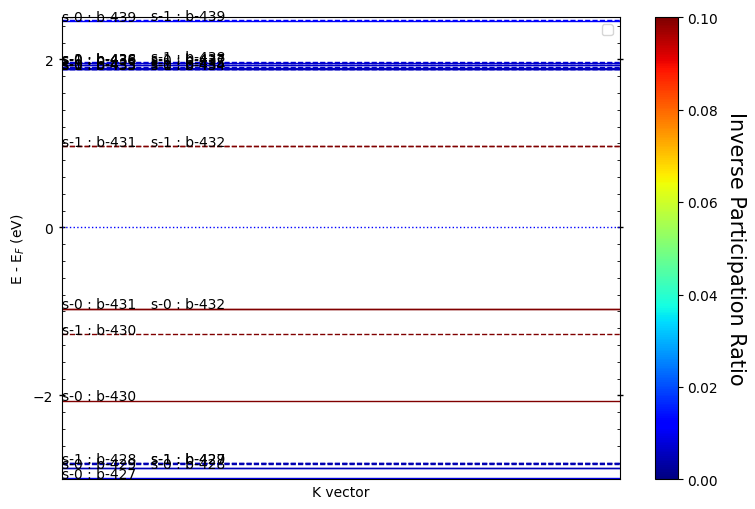
Tutorial: Inverse Participation Ratio (IPR) Analysis

Tutorial: Plotting Atomic Energy Levels

Tutorial: 2D Band Structure Visualization

Density of States Examples

Getting Started: PyProcar’s dosplot Function

Dealing with Spin in PyProcar dosplot

Comparing DOS with PyProcar

2D Fermi Surface Examples

Getting Started: PyProcar’s fermi2D Function

Dealing with Spin in PyProcar fermi2D

Rashba Spin Splitting

3D Fermi Surface Examples

Getting Started: PyProcar’s Fermi Surface 3D Visualization

Dealing with Spin in Fermi Surface 3D Visualization

De Haas-van Alphen Frequencies from Fermi Surfaces

Contents

Band Structure Examples

• Getting Started: PyProcar’s bandsplot Function
  • What You’ll Learn
  • Prerequisites
  • Overview of bandsplot Function
  • 1. Setup and Data Loading
  • 2. Core Arguments of bandsplot
  • 3. Basic Usage - Plain Mode
  • 4. Visualization Modes Overview
  • 5. Scatter/Parametric Mode - Projected Band Structures
  • 6. The Cache Argument - Speeding Up Repeated Plots
  • 7. Overlay Modes - Comparing Multiple Contributions
  • 8. Plotting Configurations - Customizing Appearance
  • 9. Saving and Output Options
  • Summary: Mastering bandsplot
• Dealing with Spin in PyProcar bandsplot
  • Understanding Spin in PyProcar
  • 1. Setup and Data Loading
  • 2. Spin-Polarized Band Structure Plotting
  • 1. Plain Mode - Basic Band Structure Plot
  • 2.2 Customizing the Plot
  • 3. Non-Collinear Band Structure Plotting
  • 4. Summary
• Compare Bands
  • Overview
  • Example: Comparing VASP and Quantum Espresso Band Structures
  • Import libraries and download example data
  • Comparing band structures
• Band Unfolding Tutorial
  • Introduction to Band Unfolding
  • Why Do We Need Band Unfolding?
  • The Physics Behind Unfolding
  • Setting Up the Environment and Data
  • Step 1: Understanding the Primitive Cell
  • Step 2: Basic Band Unfolding
  • Step 3: Exploring Different Unfolding Modes
  • Step 4: Advanced Unfolding with Projections
  • Step 5: Scatter Plot Mode
  • Summary and Key Takeaways
• Automated Band Structure Analysis (Autobands) Tutorial
  • Introduction to Autobands
  • What Does Autobands Do?
  • The Science Behind Autobands
  • Step 1: Understanding Your System
  • Step 2: Basic Autobands Analysis
  • Step 3: Understanding the Results
  • Summary and Key Takeaways
• Tutorial: Inverse Participation Ratio (IPR) Analysis
  • Introduction
  • What is the Inverse Participation Ratio?
  • Why is IPR Important?
  • Practical Applications
  • Getting Started
  • Setting up the Environment
  • Example 1: Topologically-Protected Surface States in Bi₂Se₃
  • Example 2: NV⁻ Defect States in Diamond
  • Summary and Key Takeaways
• Tutorial: Plotting Atomic Energy Levels
  • Introduction
  • What are Atomic Energy Levels?
  • System Overview: hBN with CNN Defect
  • Setting up the Environment
  • Understanding Atomic Mode in PyProcar
  • Advanced Analysis: Comparing Different Atomic Contributions
  • Summary and Key Insights
• Tutorial: 2D Band Structure Visualization
  • Introduction
  • What are 2D Band Structures?
  • System Overview: Graphene as a Model System
  • Setting up the Environment
  • Example 1: Plain Mode - Basic 2D Band Structure
  • Example 2: Parametric Mode - Atomic and Orbital Projections
  • Example 3: Property Projection Mode - Physical Properties
  • Example 4: Spin Texture Mode - Advanced Topological Materials
  • Summary and Advanced Techniques

Density of States Examples

• Getting Started: PyProcar’s dosplot Function
  • What You’ll Learn
  • Prerequisites
  • Overview of dosplot Function
  • 1. Setup and Data Loading
  • 2. Core Arguments of dosplot
  • 3. Basic Usage - Plain Mode
  • 4. Visualization Modes Overview
  • 5. Parametric Mode - Projected Density of States
  • 6. Stack Modes - Component Analysis
  • 7. Overlay Modes - Comparing Multiple Contributions
  • 8. DOS Normalization - Scaling for Comparison
  • 9. Plotting Configurations - Customizing Appearance
  • 10. Caching and Performance
  • 11. Saving and Output Options
  • Summary: Mastering dosplot
• Dealing with Spin in PyProcar dosplot
  • Understanding Spin in DOS Analysis
  • 1. Setup and Data Loading
  • 2. Spin-Polarized DOS Plotting
  • 3. Non-Collinear DOS Plotting
• Comparing DOS with PyProcar
  • Overview
  • Benefits of DOS Comparison
  • 1. Setup and Data Loading
  • 2. Basic DOS Comparison: Spin Channels

2D Fermi Surface Examples

• Getting Started: PyProcar’s fermi2D Function
  • What You’ll Learn
  • Prerequisites
  • Overview of fermi2D Function
  • 1. Setup and Data Loading
  • 2. Core Arguments of fermi2D
  • 3. Basic Usage - Plain Mode
  • 4. Visualization Modes Overview
  • 5. Parametric Mode - Projected Fermi Surface
  • 6. Plain Bands Mode - Individual Band Analysis
  • 7. Advanced Configuration and Performance
  • 8. Best Practices and Tips
  • Summary
• Dealing with Spin in PyProcar fermi2D
  • Understanding Spin in 2D Fermi Surface Analysis
  • 1. Setup and Data Loading
  • 2. Spin-Polarized Fermi Surface Plotting
  • 3. Non-Collinear Fermi Surface Plotting
  • 4. Additional fermi2D Modes for Spin Analysis
  • 5. Summary and Best Practices
• Rashba Spin Splitting
  • Introduction to Rashba Spin Splitting
  • Example: BiSb Monolayer
  • Importing PyProcar and Setting Up Data
  • Part 1: Understanding Spin Projections
  • Part 2: Visualizing Spin Textures with Arrows
  • Summary and Key Observations

3D Fermi Surface Examples

• Getting Started: PyProcar’s Fermi Surface 3D Visualization
  • What You’ll Learn
  • Prerequisites
  • Overview of FermiHandler Approach
  • 1. Setup and Data Loading
  • 2. FermiHandler Class Overview
  • 3. Creating Your First FermiHandler
  • 4. Basic Fermi Surface Plotting - Plain Mode
  • 5. Visualization Modes Overview
  • 6. Parametric Mode - Projected Fermi Surfaces
  • 8. Interactive Features - Sliders and Cross-Sections
  • 9. Plotting Configurations - Customizing 3D Appearance
  • 10. Saving and Output Options
  • Summary: Mastering PyProcar’s FermiHandler
• Dealing with Spin in Fermi Surface 3D Visualization
  • Understanding Spin in Fermi Surface Calculations
  • 1. Setup and Data Loading
  • 2. Spin-Polarized Fermi Surfaces (Collinear Magnetism)
  • 3. Non-Collinear Fermi Surfaces and Spin Texture
  • 4. Advanced Spin Analysis Techniques
  • 5. Summary: Mastering Spin in Fermi Surface Visualization
• De Haas-van Alphen Frequencies from Fermi Surfaces
  • Understanding Quantum Oscillations in Metals
  • Data Setup
  • Import Libraries and Download Data
  • Finding Extremal Cross-Sections for dHvA Frequencies
  • Summary and Conclusions