Rashba Spin Splitting
Introduction to Rashba Spin Splitting
The Rashba effect is a spin-orbit coupling phenomenon that occurs in systems with broken inversion symmetry, particularly at surfaces and interfaces. Named after Emmanuel Rashba, this effect leads to a lifting of spin degeneracy in the electronic band structure, resulting in characteristic spin-split bands.
Key Features of Rashba Spin Splitting:
Origin: Arises from the combination of:
Spin-orbit coupling (SOC)
Structural inversion asymmetry (SIA)
Electric fields perpendicular to the material surface
Band Structure Effect:
Splits originally spin-degenerate bands into two branches
Creates characteristic “camel-back” or “Mexican hat” dispersion
Each branch has opposite spin helicity
Spin Texture:
Spins are locked perpendicular to the momentum direction
Creates chiral spin textures in momentum space
Spins rotate as one moves around the Fermi surface
Physical Significance:
Important for spintronics applications
Enables electrical control of spin currents
Relevant for topological insulators and quantum computing
Example: BiSb Monolayer
In this tutorial, we’ll visualize the Rashba spin splitting in a BiSb monolayer using PyProcar. We’ll examine:
Spin textures at different energy levels
Different spin projections (Sx, Sy, Sz)
How the spin orientation changes across the Fermi surface
The BiSb monolayer is an excellent example because it exhibits strong Rashba spin splitting due to its heavy elements (Bi, Sb) and inherent inversion asymmetry.
Data Setup
First, let’s download the example files. The data includes VASP calculations with non-collinear spin treatment necessary to capture the Rashba effect.
Importing PyProcar and Setting Up Data
[1]:
# Import required libraries
from pathlib import Path
import pyprocar

CURRENT_DIR = Path(".").resolve()
REL_PATH = "data/examples/fermi2d/bisb_monolayer"
pyprocar.download_from_hf(relpath=REL_PATH, output_path=CURRENT_DIR)
DATA_DIR = CURRENT_DIR / REL_PATH
print(f"Data downloaded to: {DATA_DIR}")
c:\Users\lllang\miniconda3\envs\pyprocar\lib\site-packages\huggingface_hub\file_download.py:143: UserWarning: `huggingface_hub` cache-system uses symlinks by default to efficiently store duplicated files but your machine does not support them in C:\Users\lllang\.cache\huggingface\hub\datasets--lllangWV--pyprocar_test_data. Caching files will still work but in a degraded version that might require more space on your disk. This warning can be disabled by setting the `HF_HUB_DISABLE_SYMLINKS_WARNING` environment variable. For more details, see https://huggingface.co/docs/huggingface_hub/how-to-cache#limitations.
To support symlinks on Windows, you either need to activate Developer Mode or to run Python as an administrator. In order to activate developer mode, see this article: https://docs.microsoft.com/en-us/windows/apps/get-started/enable-your-device-for-development
  warnings.warn(message)
Data downloaded to: C:\Users\lllang\Desktop\notebooks\Notebook\01 - Projects\Pyprocar\pyprocar\examples\02-fermi2d\data\examples\fermi2d\bisb_monolayer
Part 1: Understanding Spin Projections
Energy = +0.60 eV: Above the Fermi Level
We’ll start by examining the spin texture at +0.60 eV above the Fermi level. At this energy, we’re looking at the conduction band states.
Sx Projection (No Arrows)
The x-component of spin (Sx) shows how the electron spins are oriented along the x-direction in momentum space. In Rashba systems, we expect to see characteristic patterns that reflect the chiral nature of the spin texture.
[4]:
# Plot Sx projection at +0.60 eV without arrows
# This shows the x-component of spin as a color map
pyprocar.fermi2D(
    code="vasp",
    dirname=DATA_DIR,
    energy=0.60,
    fermi=-1.1904,
    spin_texture=True,
    no_arrow=True,
    use_cache=False,
    spin_projection="x",
    plot_color_bar=True,
)
If you want more detailed logs, set verbose to 2 or more
____________________________________________________________________________________________________
 ____        ____
|  _ \ _   _|  _ \ _ __ ___   ___ __ _ _ __
| |_) | | | | |_) | '__/ _ \ / __/ _` | '__|
|  __/| |_| |  __/| | | (_) | (_| (_| | |
|_|    \__, |_|   |_|  \___/ \___\__,_|_|
       |___/
A Python library for electronic structure pre/post-processing.

Version 6.4.6 created on Mar 6th, 2025

Please cite:
- Uthpala Herath, Pedram Tavadze, Xu He, Eric Bousquet, Sobhit Singh, Francisco Muñoz and Aldo Romero.,
  PyProcar: A Python library for electronic structure pre/post-processing.,
  Computer Physics Communications 251, 107080 (2020).

- L. Lang, P. Tavadze, A. Tellez, E. Bousquet, H. Xu, F. Muñoz, N. Vasquez, U. Herath, and A. H. Romero,
  Expanding PyProcar for new features, maintainability, and reliability.,
  Computer Physics Communications 297, 109063 (2024).

Developers:
- Francisco Muñoz
- Aldo Romero
- Sobhit Singh
- Uthpala Herath
- Pedram Tavadze
- Eric Bousquet
- Xu He
- Reese Boucher
- Logan Lang
- Freddy Farah

____________________________________________________________________________________________________
### Parameters ###
dirname         : C:\Users\lllang\Desktop\notebooks\Notebook\01 - Projects\Pyprocar\pyprocar\examples\02-fermi2d\data\examples\fermi2d\bisb_monolayer
bands           : None
atoms           : None
orbitals        : None
spin comp.      : None
energy          : 0.6
rot. symmetry   : 1
origin (trasl.) : [0, 0, 0]
rotation        : [0, 0, 0, 1]
save figure     : None
spin_texture    : True
____________________________________________________________________________________________________

            There are additional plot options that are defined in a configuration file.
            You can change these configurations by passing the keyword argument to the function
            To print a list of plot options set print_plot_opts=True

            Here is a list modes : plain , plain_bands , parametric
____________________________________________________________________________________________________
Parsing KPOINTS file: C:\Users\lllang\Desktop\notebooks\Notebook\01 - Projects\Pyprocar\pyprocar\examples\02-fermi2d\data\examples\fermi2d\bisb_monolayer\KPOINTS
[INFO] 2025-06-13 12:03:38 - pyprocar.scripts.scriptFermi2D[191][fermi2D] - Shifting Fermi energy to zero: -1.1904
[DEBUG] 2025-06-13 12:03:38 - pyprocar.scripts.scriptFermi2D[200][fermi2D] - EBS:
 Electronic Band Structure
============================
Total number of kpoints   = 3600
Total number of bands    = 80
Total number of atoms    = 2
Total number of orbitals = 9
nkx,nky,nkz = (60,60,1)

Array Shapes:
------------------------
Kpoints shape  = (3600, 3)
Bands shape    = (3600, 80, 1)
Projected shape = (3600, 80, 2, 1, 9, 4)
Labels = ['s', 'py', 'pz', 'px', 'dxy', 'dyz', 'dz2', 'dxz', 'x2-y2']
Reciprocal Lattice =
 [[ 0.235   0.1357  0.    ]
 [ 0.      0.2714 -0.    ]
 [ 0.     -0.      0.0611]]

Additional information:
------------------------
Fermi Energy = -1.2184
Is Mesh = True
Has Phase = False

Initial kpoints shape: (3600, 3)
Initial bands shape: (3600, 80, 1)
Initial projected shape: (3600, 80, 2, 1, 9, 4)
WARNING: Make sure the kmesh has the correct number of kz pointswith kz=0.0 +- 0.01.
Kpoints in the kz=0.0 plane: (3600, 3)
Bands in the kz=0.0 plane: (3600, 80, 1)
Projected in the kz=0.0 plane: (3600, 80, 2, 1, 9, 4)
[INFO] 2025-06-13 12:03:38 - pyprocar.scripts.scriptFermi2D[269][fermi2D] - ebsX.projected shape after ebs_sum: (3600, 80)
[INFO] 2025-06-13 12:03:38 - pyprocar.scripts.scriptFermi2D[270][fermi2D] - ebsY.projected shape after ebs_sum: (3600, 80)
[INFO] 2025-06-13 12:03:38 - pyprocar.scripts.scriptFermi2D[271][fermi2D] - ebsZ.projected shape after ebs_sum: (3600, 80)
[DEBUG] 2025-06-13 12:04:50 - pyprocar.core.fermisurface[86][__init__] - FermiSurface.init: ...
[INFO] 2025-06-13 12:04:50 - pyprocar.core.fermisurface[87][__init__] - Kpoints.shape : (3600, 3)
[INFO] 2025-06-13 12:04:50 - pyprocar.core.fermisurface[88][__init__] - bands.shape   : (3600, 80, 1)
[INFO] 2025-06-13 12:04:50 - pyprocar.core.fermisurface[89][__init__] - spd.shape     : (3600, 80, 4)
[DEBUG] 2025-06-13 12:04:50 - pyprocar.core.fermisurface[90][__init__] - FermiSurface.init: ...Done
[INFO] 2025-06-13 12:04:50 - pyprocar.core.fermisurface[121][find_energy] - Energy   : 0.6
Band indices near iso-surface: (bands.shape=(3600, 80)) spin-0 | bands-[20 21]
[DEBUG] 2025-06-13 12:04:50 - pyprocar.core.fermisurface[332][spin_texture] - spin_texture: ...
[DEBUG] 2025-06-13 12:04:50 - pyprocar.core.fermisurface[358][spin_texture] - xlim = [-0.11358611703331413, 0.1175028805]  ylim = [-0.19673749939318966, 0.2035215525]
[DEBUG] 2025-06-13 12:04:50 - pyprocar.core.fermisurface[367][spin_texture] - Interpolating ...
[DEBUG] 2025-06-13 12:04:50 - pyprocar.core.fermisurface[367][spin_texture] - Interpolating ...
[DEBUG] 2025-06-13 12:04:50 - pyprocar.core.fermisurface[415][spin_texture] - Fermi surf. points.shape: (1063, 2)
[INFO] 2025-06-13 12:04:51 - pyprocar.core.fermisurface[419][spin_texture] - newSx.shape: (1063,)
[DEBUG] 2025-06-13 12:04:51 - pyprocar.core.fermisurface[415][spin_texture] - Fermi surf. points.shape: (87, 2)
[INFO] 2025-06-13 12:04:51 - pyprocar.core.fermisurface[419][spin_texture] - newSx.shape: (87,)
[DEBUG] 2025-06-13 12:04:51 - pyprocar.core.fermisurface[523][spin_texture] - st: ...Done

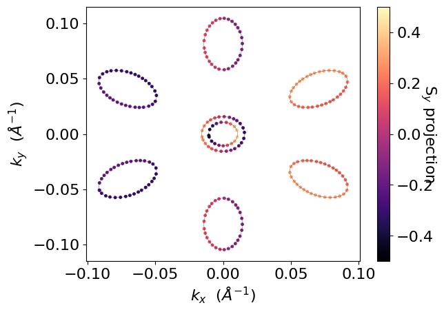
Sy Projection (No Arrows)
The y-component of spin (Sy) shows the spin orientation along the y-direction. Notice how the pattern differs from Sx - this demonstrates the chiral nature of Rashba spin textures where spins rotate as we move around in momentum space.
[5]:
# Plot Sy projection at +0.60 eV without arrows
pyprocar.fermi2D(
    code="vasp",
    dirname=DATA_DIR,
    energy=0.60,
    fermi=-1.1904,
    spin_texture=True,
    no_arrow=True,
    spin_projection="y",
    plot_color_bar=True,
)
If you want more detailed logs, set verbose to 2 or more
____________________________________________________________________________________________________
 ____        ____
|  _ \ _   _|  _ \ _ __ ___   ___ __ _ _ __
| |_) | | | | |_) | '__/ _ \ / __/ _` | '__|
|  __/| |_| |  __/| | | (_) | (_| (_| | |
|_|    \__, |_|   |_|  \___/ \___\__,_|_|
       |___/
A Python library for electronic structure pre/post-processing.

Version 6.4.6 created on Mar 6th, 2025

Please cite:
- Uthpala Herath, Pedram Tavadze, Xu He, Eric Bousquet, Sobhit Singh, Francisco Muñoz and Aldo Romero.,
  PyProcar: A Python library for electronic structure pre/post-processing.,
  Computer Physics Communications 251, 107080 (2020).

- L. Lang, P. Tavadze, A. Tellez, E. Bousquet, H. Xu, F. Muñoz, N. Vasquez, U. Herath, and A. H. Romero,
  Expanding PyProcar for new features, maintainability, and reliability.,
  Computer Physics Communications 297, 109063 (2024).

Developers:
- Francisco Muñoz
- Aldo Romero
- Sobhit Singh
- Uthpala Herath
- Pedram Tavadze
- Eric Bousquet
- Xu He
- Reese Boucher
- Logan Lang
- Freddy Farah

____________________________________________________________________________________________________
### Parameters ###
dirname         : C:\Users\lllang\Desktop\notebooks\Notebook\01 - Projects\Pyprocar\pyprocar\examples\02-fermi2d\data\examples\fermi2d\bisb_monolayer
bands           : None
atoms           : None
orbitals        : None
spin comp.      : None
energy          : 0.6
rot. symmetry   : 1
origin (trasl.) : [0, 0, 0]
rotation        : [0, 0, 0, 1]
save figure     : None
spin_texture    : True
____________________________________________________________________________________________________

            There are additional plot options that are defined in a configuration file.
            You can change these configurations by passing the keyword argument to the function
            To print a list of plot options set print_plot_opts=True

            Here is a list modes : plain , plain_bands , parametric
____________________________________________________________________________________________________
Initial kpoints shape: (3600, 3)
Initial bands shape: (3600, 80, 1)
Initial projected shape: (3600, 80, 2, 1, 9, 4)
WARNING: Make sure the kmesh has the correct number of kz pointswith kz=0.0 +- 0.01.
Kpoints in the kz=0.0 plane: (3600, 3)
Bands in the kz=0.0 plane: (3600, 80, 1)
Projected in the kz=0.0 plane: (3600, 80, 2, 1, 9, 4)
Band indices near iso-surface: (bands.shape=(3600, 80)) spin-0 | bands-[20 21]
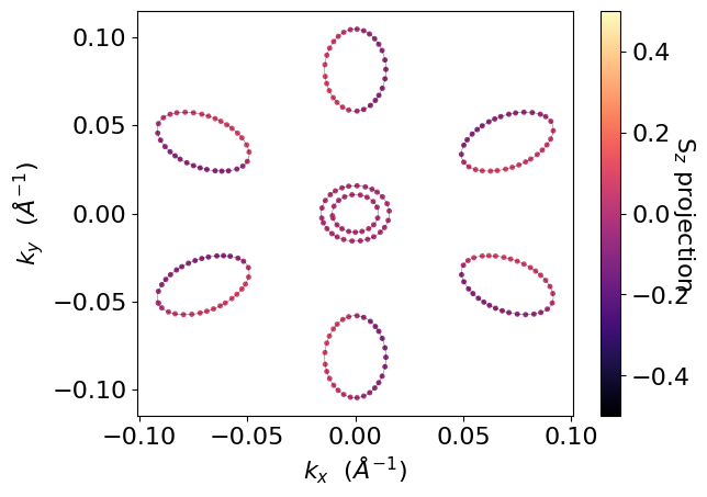
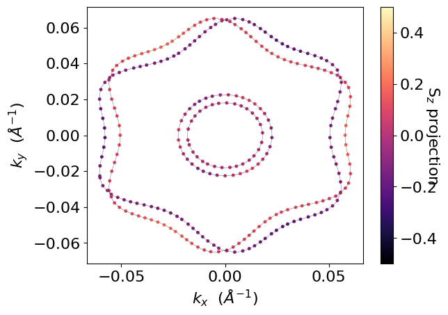
Sz Projection (No Arrows)
The z-component of spin (Sz) represents out-of-plane spin components. In 2D Rashba systems, this component is typically smaller than the in-plane components (Sx, Sy) because the Rashba effect primarily locks spins in the plane perpendicular to the electric field.
[6]:
# Plot Sz projection at +0.60 eV without arrows
pyprocar.fermi2D(
    code="vasp",
    dirname=DATA_DIR,
    energy=0.60,
    fermi=-1.1904,
    spin_texture=True,
    no_arrow=True,
    spin_projection="z",
    plot_color_bar=True,
)
If you want more detailed logs, set verbose to 2 or more
____________________________________________________________________________________________________
 ____        ____
|  _ \ _   _|  _ \ _ __ ___   ___ __ _ _ __
| |_) | | | | |_) | '__/ _ \ / __/ _` | '__|
|  __/| |_| |  __/| | | (_) | (_| (_| | |
|_|    \__, |_|   |_|  \___/ \___\__,_|_|
       |___/
A Python library for electronic structure pre/post-processing.

Version 6.4.6 created on Mar 6th, 2025

Please cite:
- Uthpala Herath, Pedram Tavadze, Xu He, Eric Bousquet, Sobhit Singh, Francisco Muñoz and Aldo Romero.,
  PyProcar: A Python library for electronic structure pre/post-processing.,
  Computer Physics Communications 251, 107080 (2020).

- L. Lang, P. Tavadze, A. Tellez, E. Bousquet, H. Xu, F. Muñoz, N. Vasquez, U. Herath, and A. H. Romero,
  Expanding PyProcar for new features, maintainability, and reliability.,
  Computer Physics Communications 297, 109063 (2024).

Developers:
- Francisco Muñoz
- Aldo Romero
- Sobhit Singh
- Uthpala Herath
- Pedram Tavadze
- Eric Bousquet
- Xu He
- Reese Boucher
- Logan Lang
- Freddy Farah

____________________________________________________________________________________________________
### Parameters ###
dirname         : C:\Users\lllang\Desktop\notebooks\Notebook\01 - Projects\Pyprocar\pyprocar\examples\02-fermi2d\data\examples\fermi2d\bisb_monolayer
bands           : None
atoms           : None
orbitals        : None
spin comp.      : None
energy          : 0.6
rot. symmetry   : 1
origin (trasl.) : [0, 0, 0]
rotation        : [0, 0, 0, 1]
save figure     : None
spin_texture    : True
____________________________________________________________________________________________________

            There are additional plot options that are defined in a configuration file.
            You can change these configurations by passing the keyword argument to the function
            To print a list of plot options set print_plot_opts=True

            Here is a list modes : plain , plain_bands , parametric
____________________________________________________________________________________________________
Initial kpoints shape: (3600, 3)
Initial bands shape: (3600, 80, 1)
Initial projected shape: (3600, 80, 2, 1, 9, 4)
WARNING: Make sure the kmesh has the correct number of kz pointswith kz=0.0 +- 0.01.
Kpoints in the kz=0.0 plane: (3600, 3)
Bands in the kz=0.0 plane: (3600, 80, 1)
Projected in the kz=0.0 plane: (3600, 80, 2, 1, 9, 4)
Band indices near iso-surface: (bands.shape=(3600, 80)) spin-0 | bands-[20 21]
Energy = -0.90 eV: Below the Fermi Level
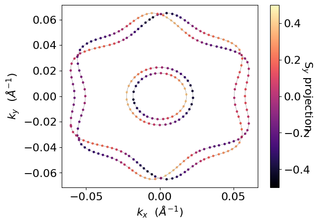
Now let’s examine the spin texture at -0.90 eV below the Fermi level. This energy corresponds to valence band states. Comparing these results with the conduction band will help us understand the electron-hole asymmetry in the Rashba effect.
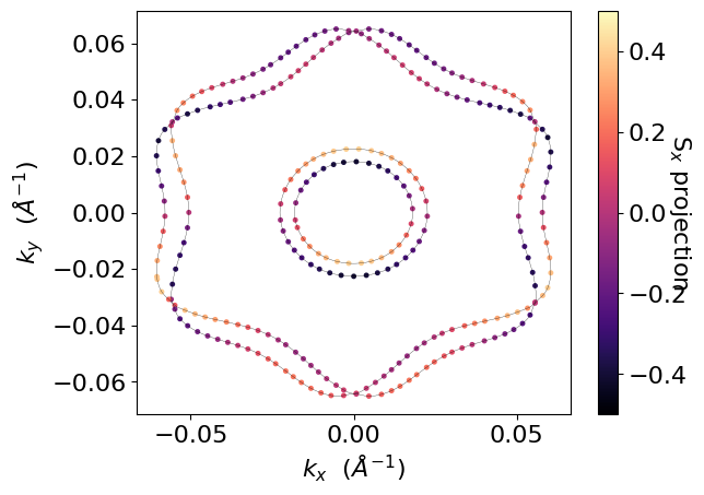
Sx Projection (No Arrows) - Valence Band
Notice how the spin texture pattern changes compared to the conduction band. This demonstrates that Rashba spin splitting affects both valence and conduction bands, but with potentially different characteristics.
[7]:
# Plot Sx projection at -0.90 eV without arrows
pyprocar.fermi2D(
    code="vasp",
    dirname=DATA_DIR,
    energy=-0.90,
    fermi=-1.1904,
    spin_texture=True,
    no_arrow=True,
    spin_projection="x",
    plot_color_bar=True,
)
If you want more detailed logs, set verbose to 2 or more
____________________________________________________________________________________________________
 ____        ____
|  _ \ _   _|  _ \ _ __ ___   ___ __ _ _ __
| |_) | | | | |_) | '__/ _ \ / __/ _` | '__|
|  __/| |_| |  __/| | | (_) | (_| (_| | |
|_|    \__, |_|   |_|  \___/ \___\__,_|_|
       |___/
A Python library for electronic structure pre/post-processing.

Version 6.4.6 created on Mar 6th, 2025

Please cite:
- Uthpala Herath, Pedram Tavadze, Xu He, Eric Bousquet, Sobhit Singh, Francisco Muñoz and Aldo Romero.,
  PyProcar: A Python library for electronic structure pre/post-processing.,
  Computer Physics Communications 251, 107080 (2020).

- L. Lang, P. Tavadze, A. Tellez, E. Bousquet, H. Xu, F. Muñoz, N. Vasquez, U. Herath, and A. H. Romero,
  Expanding PyProcar for new features, maintainability, and reliability.,
  Computer Physics Communications 297, 109063 (2024).

Developers:
- Francisco Muñoz
- Aldo Romero
- Sobhit Singh
- Uthpala Herath
- Pedram Tavadze
- Eric Bousquet
- Xu He
- Reese Boucher
- Logan Lang
- Freddy Farah

____________________________________________________________________________________________________
### Parameters ###
dirname         : C:\Users\lllang\Desktop\notebooks\Notebook\01 - Projects\Pyprocar\pyprocar\examples\02-fermi2d\data\examples\fermi2d\bisb_monolayer
bands           : None
atoms           : None
orbitals        : None
spin comp.      : None
energy          : -0.9
rot. symmetry   : 1
origin (trasl.) : [0, 0, 0]
rotation        : [0, 0, 0, 1]
save figure     : None
spin_texture    : True
____________________________________________________________________________________________________

            There are additional plot options that are defined in a configuration file.
            You can change these configurations by passing the keyword argument to the function
            To print a list of plot options set print_plot_opts=True

            Here is a list modes : plain , plain_bands , parametric
____________________________________________________________________________________________________
Initial kpoints shape: (3600, 3)
Initial bands shape: (3600, 80, 1)
Initial projected shape: (3600, 80, 2, 1, 9, 4)
WARNING: Make sure the kmesh has the correct number of kz pointswith kz=0.0 +- 0.01.
Kpoints in the kz=0.0 plane: (3600, 3)
Bands in the kz=0.0 plane: (3600, 80, 1)
Projected in the kz=0.0 plane: (3600, 80, 2, 1, 9, 4)
Band indices near iso-surface: (bands.shape=(3600, 80)) spin-0 | bands-[16 17 18 19]
Sy Projection (No Arrows) - Valence Band
[8]:
# Plot Sy projection at -0.90 eV without arrows
pyprocar.fermi2D(
    code="vasp",
    dirname=DATA_DIR,
    energy=-0.90,
    fermi=-1.1904,
    spin_texture=True,
    no_arrow=True,
    spin_projection="y",
    plot_color_bar=True,
)
If you want more detailed logs, set verbose to 2 or more
____________________________________________________________________________________________________
 ____        ____
|  _ \ _   _|  _ \ _ __ ___   ___ __ _ _ __
| |_) | | | | |_) | '__/ _ \ / __/ _` | '__|
|  __/| |_| |  __/| | | (_) | (_| (_| | |
|_|    \__, |_|   |_|  \___/ \___\__,_|_|
       |___/
A Python library for electronic structure pre/post-processing.

Version 6.4.6 created on Mar 6th, 2025

Please cite:
- Uthpala Herath, Pedram Tavadze, Xu He, Eric Bousquet, Sobhit Singh, Francisco Muñoz and Aldo Romero.,
  PyProcar: A Python library for electronic structure pre/post-processing.,
  Computer Physics Communications 251, 107080 (2020).

- L. Lang, P. Tavadze, A. Tellez, E. Bousquet, H. Xu, F. Muñoz, N. Vasquez, U. Herath, and A. H. Romero,
  Expanding PyProcar for new features, maintainability, and reliability.,
  Computer Physics Communications 297, 109063 (2024).

Developers:
- Francisco Muñoz
- Aldo Romero
- Sobhit Singh
- Uthpala Herath
- Pedram Tavadze
- Eric Bousquet
- Xu He
- Reese Boucher
- Logan Lang
- Freddy Farah

____________________________________________________________________________________________________
### Parameters ###
dirname         : C:\Users\lllang\Desktop\notebooks\Notebook\01 - Projects\Pyprocar\pyprocar\examples\02-fermi2d\data\examples\fermi2d\bisb_monolayer
bands           : None
atoms           : None
orbitals        : None
spin comp.      : None
energy          : -0.9
rot. symmetry   : 1
origin (trasl.) : [0, 0, 0]
rotation        : [0, 0, 0, 1]
save figure     : None
spin_texture    : True
____________________________________________________________________________________________________

            There are additional plot options that are defined in a configuration file.
            You can change these configurations by passing the keyword argument to the function
            To print a list of plot options set print_plot_opts=True

            Here is a list modes : plain , plain_bands , parametric
____________________________________________________________________________________________________
Initial kpoints shape: (3600, 3)
Initial bands shape: (3600, 80, 1)
Initial projected shape: (3600, 80, 2, 1, 9, 4)
WARNING: Make sure the kmesh has the correct number of kz pointswith kz=0.0 +- 0.01.
Kpoints in the kz=0.0 plane: (3600, 3)
Bands in the kz=0.0 plane: (3600, 80, 1)
Projected in the kz=0.0 plane: (3600, 80, 2, 1, 9, 4)
Band indices near iso-surface: (bands.shape=(3600, 80)) spin-0 | bands-[16 17 18 19]
Sz Projection (No Arrows) - Valence Band
[9]:
# Plot Sz projection at -0.90 eV without arrows
pyprocar.fermi2D(
    code="vasp",
    dirname=DATA_DIR,
    energy=-0.90,
    fermi=-1.1904,
    spin_texture=True,
    no_arrow=True,
    spin_projection="z",
    plot_color_bar=True,
)
If you want more detailed logs, set verbose to 2 or more
____________________________________________________________________________________________________
 ____        ____
|  _ \ _   _|  _ \ _ __ ___   ___ __ _ _ __
| |_) | | | | |_) | '__/ _ \ / __/ _` | '__|
|  __/| |_| |  __/| | | (_) | (_| (_| | |
|_|    \__, |_|   |_|  \___/ \___\__,_|_|
       |___/
A Python library for electronic structure pre/post-processing.

Version 6.4.6 created on Mar 6th, 2025

Please cite:
- Uthpala Herath, Pedram Tavadze, Xu He, Eric Bousquet, Sobhit Singh, Francisco Muñoz and Aldo Romero.,
  PyProcar: A Python library for electronic structure pre/post-processing.,
  Computer Physics Communications 251, 107080 (2020).

- L. Lang, P. Tavadze, A. Tellez, E. Bousquet, H. Xu, F. Muñoz, N. Vasquez, U. Herath, and A. H. Romero,
  Expanding PyProcar for new features, maintainability, and reliability.,
  Computer Physics Communications 297, 109063 (2024).

Developers:
- Francisco Muñoz
- Aldo Romero
- Sobhit Singh
- Uthpala Herath
- Pedram Tavadze
- Eric Bousquet
- Xu He
- Reese Boucher
- Logan Lang
- Freddy Farah

____________________________________________________________________________________________________
### Parameters ###
dirname         : C:\Users\lllang\Desktop\notebooks\Notebook\01 - Projects\Pyprocar\pyprocar\examples\02-fermi2d\data\examples\fermi2d\bisb_monolayer
bands           : None
atoms           : None
orbitals        : None
spin comp.      : None
energy          : -0.9
rot. symmetry   : 1
origin (trasl.) : [0, 0, 0]
rotation        : [0, 0, 0, 1]
save figure     : None
spin_texture    : True
____________________________________________________________________________________________________

            There are additional plot options that are defined in a configuration file.
            You can change these configurations by passing the keyword argument to the function
            To print a list of plot options set print_plot_opts=True

            Here is a list modes : plain , plain_bands , parametric
____________________________________________________________________________________________________
Initial kpoints shape: (3600, 3)
Initial bands shape: (3600, 80, 1)
Initial projected shape: (3600, 80, 2, 1, 9, 4)
WARNING: Make sure the kmesh has the correct number of kz pointswith kz=0.0 +- 0.01.
Kpoints in the kz=0.0 plane: (3600, 3)
Bands in the kz=0.0 plane: (3600, 80, 1)
Projected in the kz=0.0 plane: (3600, 80, 2, 1, 9, 4)
Band indices near iso-surface: (bands.shape=(3600, 80)) spin-0 | bands-[16 17 18 19]
Part 2: Visualizing Spin Textures with Arrows
Understanding the Chiral Nature of Rashba Spin Splitting
The previous plots showed spin projections as color maps, but to truly understand the Rashba effect, we need to visualize the spin texture - how the spin vectors are oriented in momentum space. This is where the arrows become essential.
Energy = +0.60 eV: Sx Projection with Arrows
Now let’s add arrows to visualize the actual spin directions. The arrows represent the in-plane spin vectors, while the color map shows the Sx projection. This combination reveals the characteristic chiral spin texture of Rashba systems.
[11]:
# Plot Sx projection at +0.60 eV with arrows showing spin texture
# The arrows reveal the chiral nature of the Rashba spin texture
pyprocar.fermi2D(
    code="vasp",
    dirname=DATA_DIR,
    energy=0.60,
    fermi=-1.1904,
    spin_texture=True,
    spin_projection="x",
    arrow_size=0.5,
    arrow_density=6,
    plot_color_bar=True,
)
If you want more detailed logs, set verbose to 2 or more
____________________________________________________________________________________________________
 ____        ____
|  _ \ _   _|  _ \ _ __ ___   ___ __ _ _ __
| |_) | | | | |_) | '__/ _ \ / __/ _` | '__|
|  __/| |_| |  __/| | | (_) | (_| (_| | |
|_|    \__, |_|   |_|  \___/ \___\__,_|_|
       |___/
A Python library for electronic structure pre/post-processing.

Version 6.4.6 created on Mar 6th, 2025

Please cite:
- Uthpala Herath, Pedram Tavadze, Xu He, Eric Bousquet, Sobhit Singh, Francisco Muñoz and Aldo Romero.,
  PyProcar: A Python library for electronic structure pre/post-processing.,
  Computer Physics Communications 251, 107080 (2020).

- L. Lang, P. Tavadze, A. Tellez, E. Bousquet, H. Xu, F. Muñoz, N. Vasquez, U. Herath, and A. H. Romero,
  Expanding PyProcar for new features, maintainability, and reliability.,
  Computer Physics Communications 297, 109063 (2024).

Developers:
- Francisco Muñoz
- Aldo Romero
- Sobhit Singh
- Uthpala Herath
- Pedram Tavadze
- Eric Bousquet
- Xu He
- Reese Boucher
- Logan Lang
- Freddy Farah

____________________________________________________________________________________________________
### Parameters ###
dirname         : C:\Users\lllang\Desktop\notebooks\Notebook\01 - Projects\Pyprocar\pyprocar\examples\02-fermi2d\data\examples\fermi2d\bisb_monolayer
bands           : None
atoms           : None
orbitals        : None
spin comp.      : None
energy          : 0.6
rot. symmetry   : 1
origin (trasl.) : [0, 0, 0]
rotation        : [0, 0, 0, 1]
save figure     : None
spin_texture    : True
____________________________________________________________________________________________________

            There are additional plot options that are defined in a configuration file.
            You can change these configurations by passing the keyword argument to the function
            To print a list of plot options set print_plot_opts=True

            Here is a list modes : plain , plain_bands , parametric
____________________________________________________________________________________________________
Initial kpoints shape: (3600, 3)
Initial bands shape: (3600, 80, 1)
Initial projected shape: (3600, 80, 2, 1, 9, 4)
WARNING: Make sure the kmesh has the correct number of kz pointswith kz=0.0 +- 0.01.
Kpoints in the kz=0.0 plane: (3600, 3)
Bands in the kz=0.0 plane: (3600, 80, 1)
Projected in the kz=0.0 plane: (3600, 80, 2, 1, 9, 4)
Band indices near iso-surface: (bands.shape=(3600, 80)) spin-0 | bands-[20 21]

Energy = -0.90 eV: Sx Projection with Arrows
Compare this valence band spin texture with the conduction band above. Notice how the chirality and overall pattern may differ, illustrating the complexity of Rashba spin splitting across different energy levels.
[12]:
# Plot Sx projection at -0.90 eV with arrows showing spin texture
pyprocar.fermi2D(
    code="vasp",
    dirname=DATA_DIR,
    energy=-0.90,
    fermi=-1.1904,
    spin_texture=True,
    spin_projection="x",
    arrow_size=0.3,
    arrow_density=6,
    plot_color_bar=True,
)
If you want more detailed logs, set verbose to 2 or more
____________________________________________________________________________________________________
 ____        ____
|  _ \ _   _|  _ \ _ __ ___   ___ __ _ _ __
| |_) | | | | |_) | '__/ _ \ / __/ _` | '__|
|  __/| |_| |  __/| | | (_) | (_| (_| | |
|_|    \__, |_|   |_|  \___/ \___\__,_|_|
       |___/
A Python library for electronic structure pre/post-processing.

Version 6.4.6 created on Mar 6th, 2025

Please cite:
- Uthpala Herath, Pedram Tavadze, Xu He, Eric Bousquet, Sobhit Singh, Francisco Muñoz and Aldo Romero.,
  PyProcar: A Python library for electronic structure pre/post-processing.,
  Computer Physics Communications 251, 107080 (2020).

- L. Lang, P. Tavadze, A. Tellez, E. Bousquet, H. Xu, F. Muñoz, N. Vasquez, U. Herath, and A. H. Romero,
  Expanding PyProcar for new features, maintainability, and reliability.,
  Computer Physics Communications 297, 109063 (2024).

Developers:
- Francisco Muñoz
- Aldo Romero
- Sobhit Singh
- Uthpala Herath
- Pedram Tavadze
- Eric Bousquet
- Xu He
- Reese Boucher
- Logan Lang
- Freddy Farah

____________________________________________________________________________________________________
### Parameters ###
dirname         : C:\Users\lllang\Desktop\notebooks\Notebook\01 - Projects\Pyprocar\pyprocar\examples\02-fermi2d\data\examples\fermi2d\bisb_monolayer
bands           : None
atoms           : None
orbitals        : None
spin comp.      : None
energy          : -0.9
rot. symmetry   : 1
origin (trasl.) : [0, 0, 0]
rotation        : [0, 0, 0, 1]
save figure     : None
spin_texture    : True
____________________________________________________________________________________________________

            There are additional plot options that are defined in a configuration file.
            You can change these configurations by passing the keyword argument to the function
            To print a list of plot options set print_plot_opts=True

            Here is a list modes : plain , plain_bands , parametric
____________________________________________________________________________________________________
Initial kpoints shape: (3600, 3)
Initial bands shape: (3600, 80, 1)
Initial projected shape: (3600, 80, 2, 1, 9, 4)
WARNING: Make sure the kmesh has the correct number of kz pointswith kz=0.0 +- 0.01.
Kpoints in the kz=0.0 plane: (3600, 3)
Bands in the kz=0.0 plane: (3600, 80, 1)
Projected in the kz=0.0 plane: (3600, 80, 2, 1, 9, 4)
Band indices near iso-surface: (bands.shape=(3600, 80)) spin-0 | bands-[16 17 18 19]

Summary and Key Observations
What We’ve Learned About Rashba Spin Splitting
Through this tutorial, we’ve visualized several key aspects of the Rashba effect in BiSb monolayer:
Energy-Dependent Spin Textures:
Conduction band (+0.60 eV) and valence band (-0.90 eV) show different spin texture patterns
This demonstrates that Rashba splitting affects multiple bands with varying characteristics
Spin Component Analysis:
Sx and Sy projections show strong, complementary patterns reflecting the in-plane chiral spin texture
Sz projection typically shows weaker signals, as expected for 2D Rashba systems where spins are primarily locked in-plane
Chiral Spin Textures:
The arrow plots reveal the characteristic helical or chiral nature of Rashba spin textures
Spins rotate as you move around in momentum space, with a definite handedness (chirality)
This chirality is what makes Rashba systems promising for spintronics applications
Momentum-Space Patterns:
The spin textures often show circular or hexagonal symmetries reflecting the underlying crystal structure
The patterns are energy-dependent, showing the complex nature of spin-orbit coupling effects